Inflation of Universe by Nonlinear Electrodynamics
S. I. Kruglov 1
Department of Physics, University of Toronto, 60 St. Georges St., Toronto, ON M5S 1A7, Canada
Department of Chemical and Physical Sciences, University of Toronto, 3359 Mississauga Road North, Mississauga, ON L5L 1C6, Canada
Abstract
Nonlinear electrodynamics with two dimensional parameters is stud-ied. The range of electromagnetic fields when principles of causality, unitarity and the classical stability hold are obtained. A singularity of the electric field at the center of charges is absent within our model and there are corrections to the Coulomb law as r → ∞. The uni-verse inflation takes place in the background of stochastic magnetic fields. The second stage of the universe evolution is the radiation era so that the graceful exit exists. We estimated the spectral index, the tensor-to-scalar ratio, and the running of the spectral index that are in an approximate agreement with the PLANK and WMAP data.
1
Introduction
The universe inflation can be explained by modifying the general relativity (GR) [1], [2]. But it is possible to explain the inflation of the universe by coupling GR with nonlinear electromagnetic fields [3], [4], [5], [6], [7], [8], [9], [10], [11], [12], [13], [14]. In the early time of the universe evolution electromagnetic fields were very strong and quantum corrections should be taken into account [15] and, as a result, Maxwell’s electrodynamics becomes nonlinear electrodynamics (NED) [16], [17], [18]. First NED, without singu-larities of point-like charges, was proposed by Born and Infeld [19]. In this paper we study NED that for weak fields leads to the Maxwell limit. We assume that the universe filled by the stochastic magnetic background.
Stochastic fluctuations in electron-positron plasma can lead to a stochas-tic magnestochas-tic field [20], [21]. Thus, in the early stage of the radiation-dominated era the early universe was filled by a strong low-frequency random
1E-mail: [email protected]
1
magnetic fields. It is known that there are magnetic fields in the order of
B = 10−6 G in our galaxy and other spiral galaxies [22], and they possess the primordial origin. Such magnetic fields can be generated by means of the galactic dynamo mechanism. According to the galactic dynamo theory angular momentum energy is transferred into magnetic energy. This mech-anism needs the existence of weak seed fields in the order of B = 10−19 G at the epoch of the galaxy formation. Such seed magnetic fields may be the result of thermal fluctuations of the primordial plasma and the long wave-length fluctuations can be reconnected. Then the magnetic energy may be redistributed over larger scales. It should be noted that the origin of cosmic magnetism on the largest scales of galaxies and galaxy clusters is still an open problem [23]. We consider the magnetic background because the elec-tric field is screened by the charged primordial plasma [21]. In the standard cosmological model the asymmetry in the direction is absent, hBi = 0, and there is no the directional effects.
The structure of the paper is as follows. In Sect. 2 we consider a NED model with two dimensional parametersβ,γ, and the causality and unitarity principles are studied. We analyze field equations and their dual invariance in Sect. 3. It is demonstrated that there is no singularity of the electric field at the origin of the point-like charges and the electric field possesses the maximum. There are corrections to Coulomb’s law in the order of O(r−6). We estimate the model parameters β and γ by the requirement that at the weak field limit our model is converted into QED with one loop correction. In Sect. 4 we investigate the cosmology of the universe which is filled by stochastic magnetic fields. The energy density and pressure as the functions of the scale factor are obtained. It was demonstrated that the singularity of the Ricci scalar is absent. The evolution of the universe is studied in Sect. 5. The dependence of the scale factor on the time is found. The bound on the speed of sound which guarantees the classical stability and causality is calculated. We evaluate in Sect. 6 the cosmological parameters (the spectral index ns, the tensor-to-scalar ratio r, and the running of the spectral index αs). It is shown that they agreed approximately with the PLANK and WMAP data. Section 7 is a conclusion.
We use the units with c = ¯h = ε0 = µ0 = 1. The metric signature is
2
The NED model
Here, we propose NED with the Lagrangian density given by
L =− F
(1 + 2βF)3/2 +
γ
2G
2
, (1)
where F = (1/4)FµνFµν = (B2−E2)/2, G = (1/4)FµνF˜µν = B·E ( ˜Fµν =
µναβF
αβ/2 is a dual tensor), Fµν =∂µAν −∂νAµ, and β (β >0), γ (γ >0) are dimensional parameters. The symmetrical stress-tensor following from Eq. (1) is
Tµν =LFFµαFνα+
1 2LG
FµαF˜να+FναF˜µα
−gµνL
= (βF −1)F α µ Fνα (1 + 2βF)5/2 +
1 2γG
FµαF˜να+FναF˜µα
−gµνL, (2)
where LF =∂L/∂F, LG =∂L/∂G. Making use of Eq. (2) we find the trace of the stress-tensor
T ≡ Tµµ= 12βF
2
(1 + 2βF)5/2 + 2γG
2. (3)
In Maxwell’s electrodynamicsβ →0,γ →0 andL → −F so that the energy-momentum tensor is traceless, T →0. Because the dimensional parameters are present in the model the scale invariance is violated and the stress-tensor is not traceless. From Eq. (1) one obtains the energy density ρ and the pressure pas follows:
ρ=−L −E2LF+GLG =
(1−βF)E2
(1 + 2βF)5/2 +
F
(1 + 2βF)3/2 +
1 2γG
2, (4)
p=L+E
2−2B2
3 LF−GLG =−
F
(2βF+ 1)3/2+
(E2−2B2)(βF −1)
3(2βF+ 1)5/2 −
1 2γG
2.
(5)
2.1
The causality and unitarity principles
not tachyons in the theory spectrum. The unitarity principle guarantees the absence of ghosts. Both principles lead to the inequalities [24]:
LF ≤0, LF F ≥0, LGG ≥0,
LF + 2F LF F ≤0, 2F LGG− LF ≥0. (6)
By virtue of Eq. (1) one obtains
LF =
βF −1
(1 + 2βF)5/2, LGG =γ, 2F LGG− LF = 2Fγ+
1−βF (1 + 2βF)5/2,
LF + 2F LF F =
−4(βF)2+ 11βF −1
(1 + 2βF)7/2 , LF F =
3β(2−βF)
(1 + 2βF)7/2. (7)
Making use of Eqs. (6) and (7), in the case of γ = 0, B = 0, we obtain |E| ≤ q1/β which is satisfied because the maximum of the electric field is given by |Emax| =
q
1/β (see Eq. (19)). If γ = 0, E = 0, one has |B| ≤q(11−√105)/(4β)≈0.434/√β.
3
Electromagnetic field equations
With the help of Eq. (1) we find field equations
∂µ
LFFµν +LGF˜µν
= 0. (8)
Making use of Eqs. (1) and (8) we obtain
∂µ
(βF −1)Fµν
(1 + 2βF)5/2 +γGF˜
µν !
= 0. (9)
Using the equation D=∂L/∂E, we find the electric displacement field
D = 1−βF
(1 + 2βF)5/2E+γGB. (10)
The magnetic field H=−∂L/∂B is given by
H= 1−βF
We use the decomposition of Eqs. (10) and (11) as follows [25]:
Di =εijEj +νijBj, Hi = (µ−1)ijBj−νjiEj. (12)
Making use of Eqs. (10), (11) and (12) one finds
εij =δijε, (µ−1)ij =δijµ−1, νji =δijν,
ε= 1−βF
(1 + 2βF)5/2, µ
−1 =ε= 1−βF
(1 + 2βF)5/2, ν =γG. (13)
Field equation (9), by virtue of Eqs. (10) and (11), can be represented as the Maxwell equations
∇ ·D= 0, ∂D
∂t − ∇ ×H= 0. (14)
Because εij, (µ−1)ij, and νji depend on electromagnetic fields, Eq. (14) are nonlinear Maxwell’s equations. Using the Bianchi identity ∂µF˜µν = 0, we obtain the second pair of Maxwell’s equations
∇ ·B= 0, ∂B
∂t +∇ ×E= 0. (15)
With the aid Eqs. (10) and (11) we find
D·H= (ε2−ν2)E·B+εν(B2−E2). (16) The dual symmetry is broken as D·H6=E·B [26]. In BI electrodynamics and in Maxwell’s electrodynamics (ε = 1, ν = 0) the dual symmetry holds. In quantum electrodynamics with quantum corrections and in generalized BI electrodynamics [27] the dual symmetry is violated.
3.1
The fields of point-like electric charges
When the source is a point-like electric charge qe, the electric displacement field obeys the equation
∇ ·D= 4πqeδ(r). (17)
Making use of Eq. (10) at B = 0 the solution to Eq. (17) is given by
E(2 +βE2)
2(1−βE2)5/2 =
qe
In accordance with Eq. (18) as r →0 the solution is
E(0) = s
1
β. (19)
Equation (19) shows the maximum of the electric field in the center of charged particles similar to BI electrodynamics. Thus, at the origin of the point-like charges there is no singularity of the electric field unpoint-like the Maxwell electrodynamics. Let us introduce unitless variables
x= r
2
qe √
β, y=
q
βE. (20)
Then Eq. (18) can be written as follows:
y(2 +y2)
2(1−y2)5/2 =
1
x. (21)
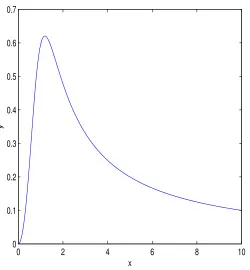
The function y(x) is depicted in Fig. 1. The approximate real and positive
0 10 20 30 40 50 0
0.1 0.2 0.3 0.4 0.5 0.6 0.7 0.8
x
y
Figure 1: The function y(x).
Table 1:
x 1 2 3 4 5 6 7 8 9 10
y 0.475 0.344 0.267 0.217 0.181 0.155 0.135 0.120 0.107 0.097
asymptotic
y= 1
x −
3
x3 +O(x
−5). (22)
Making use of Eqs. (20) and (22) we obtain the electric field as r→ ∞
E(r) = qe
r2 −
3βq3
e
r6 +O(r
−10
). (23)
According to Eq. (23) Coulomb’s law possesses corrections in the order of O(r−6). Atβ = 0 one finds the Coulomb law E =qe/r2 similar to Maxwell’s electrodynamics. Making use of Eq. (21), one finds the asymptotic of y(x) as x→0
y(x) = 1−0.59x0.4 x→0. (24)
With the help of Eq. (20), we obtain the asymptotic
E(r) = √1
β −
0.59r0.8
q0.4
e β0.7
r→0. (25)
Equation (25) at r = 0 leads to Eq. (19) and gives the electric field over short distances.
3.2
Estimation of parameters
β
and
γ
Now, we define the model parameters β and γ by the requirement that at the weak field limit our model is converted into the Heisenberg−Euler elec-trodynamics. Expanding Lagrangian (1) at small value βF 1, we have
L=−F + 3βF2− 15 2 β
2F3
+O(βF)4+ γ 2G
2
. (26)
The QED Lagrangian with one loop correction (the Heisenberg−Euler La-grangian) is given by [28]
LHE =−F +c1F2+c2G2, c2 =
14α2
45m4
e
, c1 =
8α2
45m4
e
where the coupling constant α = e2/(4π) ≈ 1/137 and the electron mass
me= 0.51 MeV. By identifying Eqs. (26) and (27) we obtain
β = 8α
2
135m4
e
= 4.6×10⁻⁵ MeV−4, γ = 28α
2
45m4
e
= 4.9×10⁻⁴ MeV−4. (28)
4
Cosmology
The action of GR coupled to electromagnetic fields is given by
S =
Z
d4x√−g
1
2κ2R+L
, (29)
where MP l = κ−1 is the reduced Planck mass and R is the Ricci scalar. By varying the action (29) we obtain the Einstein and electromagnetic field equations
Rµν −
1
2gµνR=−κ
2T
µν, (30)
∂µ √
−gFµν(βF −1) (2βF+ 1)5/2
!
= 0. (31)
The squared of the line element of homogeneous and isotropic spacetime is given by
ds2 =−dt2+a(t)2dx2+dy2+dz2, (32)
a(t) is a scale factor. We assume that the cosmic background filled by stochas-tic magnestochas-tic fields. The averaged magnestochas-tic fields (that are sources of gravita-tional fields) which guaranty the isotropy of the Friedman−Robertson−Walker (FRW) spacetime obey the equations [29]
hBi= 0, hEiBji= 0, hBiBji= 1 3B
2g
ij. (33)
Here, the brackets h.i mean an average over a volume but for a simplicity in the following we will omit the brackets h.i. The NED energy-momentum tensor with Eqs. (33) represents a perfect fluid [8]. The Friedman equation is given as follows:
3¨a
a =−
κ2
2 (ρ+ 3p), (34)
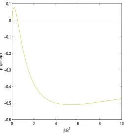
universe acceleration holds. According to the standard cosmological model, an isotropic symmetry is guarantied if hBi= 0. Making use of Eqs. (4) and (5) we find (in the case of E= 0)
ρ+ 3p=−B
2(2βB2−1)
(1 +βB2)5/2 . (35)
The plot of β(ρ+ 3p) as a function of βB2 is represented by Fig. 2. If
0 2 4 6 8 10
−0.6 −0.5 −0.4 −0.3 −0.2 −0.1 0 0.1
β B2
β
(
ρ
+3p)
Figure 2: The functionβ(ρ+ 3p) versus βB2.
βB2 > 0.5 one has ρ+ 3p < 0 and the universe acceleration occurs. As a result, the strong magnetic fields lead to the inflation of the universe. Consider the conservation of the stress-tensor, ∇µT
µν = 0,
˙
ρ+ 3a˙
With the aid of Eqs. (4) and (5) if E= 0, one obtains
ρ= B
2
2 (1 +βB2)3/2, ρ+p=
B2(2−βB2)
3 (1 +βB2)5/2. (37)
Taking into account Eq. (37), one finds the solution to Eq. (36)
B(t) = B0
a2(t), (38)
whereB0 is the value of the magnetic field which corresponds toa(t) = 1. The
scale factor a(t) increases due to the universe expansion and the magnetic field B(t) decreases. With the help of Eqs. (37) and (38) we obtain the energy density and pressure
ρ(t) = a
2(t)B2 0
2 (a4(t) +βB2 0)
3/2, p(t) =
a2(t)B2
0(a4(t)−5βB02)
6 (a4(t) +βB2 0)
5/2 . (39)
Making use of Eqs. (39) one finds
lim
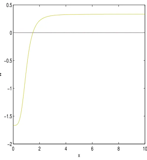
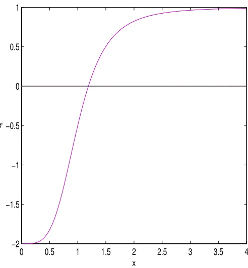
a(t)→0ρ(t) = lima(t)→0p(t) = a(limt)→∞ρ(t) = a(limt)→∞p(t) = 0. (40) Equation (40) shows that there are not singularities of the density of the energy and pressure as a(t) → 0 and a(t) → ∞. The plot of the equation of state (EoS) w =p(t)/ρ(t) versus x =a(t)/(βB02)1/4 is depicted in Fig. 3. Making use of Eqs. (39) we obtain
lim
x→∞w= limx→∞
x4−5
3(x4+ 1) =
1
3. (41)
In accordance with Eq. (41) the EoS corresponds to the ultra-relativistic behaviour [30] as a(t) → ∞. The de Sitter spacetime, w = −1, is realized for x= 1/√4
2≈0.84. From Eq. (3) and (30) we find the Ricci scalar
R=κ2T = 3κ
2βB4
(1 +βB2)5/2 =κ
2[ρ(t)−3p(t)]. (42)
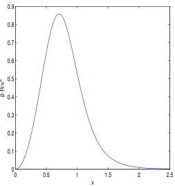
The βR/κ2 as a function of [1/(βB2
0)]1/4a is depicted in Fig. 4. Making use
of Eqs. (40) and (42) one finds
lim
0 2 4 6 8 10 −2
−1.5 −1 −0.5 0 0.5
x
w
Figure 3: The function wversus x=a/(βB2 0)1/4.
In accordance with Eq. (43) there is not a singularity of the Ricci scalar. The Kretschmann scalar RµναβRµναβ and the Ricci tensor squared RµνRµν can be expressed in the form of combinations of κ4ρ2, κ4ρp, and κ4p2 [11]. Then they vanish, in accordance with Eq. (40), as a(t)→0 and a(t)→ ∞. During the evolution of the universe the scale factor increases as t → ∞ and spacetime becomes flat. Equations (35) and (38) show that the universe acceleration takes place at a(t)<(2β)1/4√B
0 ≈1.19β1/4
√
B0.
5
Evolution of the universe
For the three dimensional flat universe the second Friedman equation is
a˙
a
2
= κ
2ρ
0 0.5 1 1.5 2 2.5 0
0.1 0.2 0.3 0.4 0.5 0.6 0.7 0.8 0.9
x
β
R/
κ
2
Figure 4: The function βR/κ2 versus x≡a/(βB2 0)1/4.
Making use of Eqs. (37), (38) and (44), one obtains
˙
a = κB0a
2
√
6(a4+βB2 0)3/4
. (45)
Introducing the unitless variable x=a/(β1/4√B0), Eq. (45) is rewritten as
˙
x= κx
2
√
6β(x4+ 1)3/4. (46)
The plot of the function y ≡ √6βx/κ˙ is depicted in Fig. 5. According to Fig. 5 at the initial time the universe inflation takes place, ( ˙y > 0), then the graceful exit occurs at the point x = √4
2 ( ˙y= 0) and after the universe decelerates. From Eq. (46) we obtain
Z x
(x4+ 1)3/4
x2 dx=
κ
√ 6β
Z t
0
0 2 4 6 8 10 0
0.1 0.2 0.3 0.4 0.5 0.6 0.7
x
y
Figure 5: The functiony ≡√6βx/κ˙ versus x.
Calculating the integrals in Eq. (47) one arrives at
x32F1
1
4, 3 4;
7 4;−x
4− (x4+ 1)3/4
x
−32F1
1
4, 3 4;
7 4;−
4+ (4+ 1)3/4
=
κt
√
6β, (48)
2F1(a, b;c;z) is the hypergeometric function, corresponds to the beginning
of the universe inflation. We can study the evolution of the universe inflation from Eq. (48). To obtain the asymptotic of the scale factor as t → ∞ we explore the relation [32]
2F1(a, b;c;z) =
Γ(c)Γ(b−a) Γ(b)Γ(c−a)(−z)
−a
2F1(a,1−c+a; 1−b+a; 1/z)
+Γ(c)Γ(a−b) Γ(a)Γ(c−b)(−z)
−b
Making use of Eq. (49) one obtains
2F1(1/4,3/4; 7/4;−x4) =
Γ(7/4)Γ(1/2) Γ(3/4)Γ(3/2)(x)
−1
2F1(1/4,−1/2; 1/2;−1/x4)
+Γ(7/4)Γ(−1/2) Γ(1/4)Γ(1) (x)
−3
2F1(3/4,0; 3/2;−1/x4). (50)
Expanding the hypergeometric functions in 1/x4 → 0 in the leading order,
we find from Eq. (48) 1.66x2 ≈κt/√6β and the scale factor is given by
a(t)≈0.5qκB0t t → ∞. (51)
Equation (51) shows that the behavior of the scale factor as t → ∞ cor-responds to the radiation era. Let us consider the deceleration parameter, making use of Eqs. (34), (37), (38) and (44)
q=− ¨aa
( ˙a)2 =
x4−2
x4+ 1. (52)
In Fig. (6) the deceleration parameter q versus x=a/(βB2
0)1/4 is depicted.
The inflation (q <0) occurs until the graceful exit pointx=√4
2≈1.19. The deceleration parameter becomes zero at x = √4
2 and then the deceleration phase (q >0) takes place. The similar behavior of the scale factor occurs in another model proposed in [14].
Now we estimate the amount of the inflation using the definition of e-folding [33]
N = lna(tend)
a(tin)
, (53)
wheretinis an initial time andtend is the final time of the inflation. Using the graceful exit point x≈1.19 one obtainsa(tend)≈1.19b (b≡β1/4
√
B0). It is
known that the horizon and flatness problems may be solved when e-folding is N ≈ 70 [33]. From Eq. (53) we obtain the scale factor corresponding to the initial time of the inflation
a(tin) = 1.19b
exp(70) ≈4.7×10 −31
b. (54)
Then ≈ 4.7×10⁻³¹. We use the units κ = √8πG = 4.1×10⁻²⁸ eV−1,
0 0.5 1 1.5 2 2.5 3 3.5 4 −2
−1.5 −1 −0.5 0 0.5 1
x
q
Figure 6: The function q versus x=a/(βB2 0)1/4.
the duration of the inflationary period. Then one obtains κ/√6β = 2.47× 10⁻¹⁴eV = 37 s−1. Using the valuex=√4
5.1
The speed of sound and causality
The causality holds when the speed of the sound is less than the local light speed, cs ≤ 1 [31]. If the square sound speed is positive (c2s >0) a classical stability is guarantied. From Eqs. (4) and (5) one can obtain the sound speed squared (for the case of E = 0)
c2s = dp
dρ =
5β2B4−23βB2+ 2)
3(βB2+ 1)(2−βB2). (55)
The classical stability requirement c2
s >0 gives the bound
0< βB2 < 23−
√ 489
10 ≈0.09 or 2< βB
2
< 23 +
√ 489
10 ≈4.5. (56)
The causality c2
s ≤1 requires that
0≤βB2 <2 or βB2 ≥ 13 + √
201
8 ≈3.4. (57)
Equations (56) and (57) give the bounds
0≤βB2 < 23−
√ 489
10 or
13 +√201
8 ≤βB
2 < 23 +
√ 489
10 . (58)
The principles of causality and unitarity studied in Sec. 2, and Eqs. (58) take place when the inequality is satisfied at the deceleration phase of the universe evolution:
0≤βB2 < 23−
√ 489
10 ≈0.09. (59)
The acceleration phase is realized at βB2 > 0.5 and the classical stability,
causality and unitarity are violated in this phase.
6
The cosmological parameters
From Eqs. (4) and (5) at E = 0 we obtain the equations
p=−ρ+ 2ρ(2−βB
2)
4ρ2(βB2+ 1)3 −B4 = 0. (61) One can find the solution (for βB2 as a function ofβρ) to the cubic equation
(61) and to place it to Eq. (60) obtaining the equation of state for perfect fluid
p=−ρ+f(ρ). (62)
If the condition |f(ρ)/ρ| 1 is satisfied the expressions for the spectral index ns, the tensor-to-scalar ratio r, and the running of the spectral index
αs =dns/dlnk are [34]
ns ≈1−6
f(ρ)
ρ , r≈24
f(ρ)
ρ , αs≈ −9
f(ρ)
ρ
!2
. (63)
From Eqs. (63) we find the equation
r= 4(1−ns) = 8 √
−αs. (64)
In accordance with the PLANCK experiment [35] and WMAP data [36], [37] we have the result
ns= 0.9603±0.0073 (68%CL), r <0.11 (95%CL),
αs =−0.0134±0.0090 (68%CL). (65)
When we take r = 0.13, using Eqs. (65), the values for the spectral index is ns = 0.9675 and the running of the spectral index is αs = −2.64×10⁻⁴. Using Eq. (63) one obtains the value f(ρ)/ρ≈0.005 and from Eq. (60) the relation is
f(ρ)
ρ =
2(2−βB2)
3(βB2+ 1). (66)
Then from Eq. (66) we find the value (for r = 0.13) of the magnetic field
B ≈1.4/√β ≈206 MeV2 ≈1012 T (see subsection 3.2) that corresponds to the inflation phase with the maximum of the energy density βρ≈0.192.
7
Conclusion
range of electromagnetic fields when causality, the classical stability and uni-tarity hold, were obtained. The dual symmetry is broken in this model because of dimensional parameters β and γ. It was shown that corrections to Coulomb’s law are in the order of O(r−6). The magnetic universe with
a stochastic background hB2i 6= 0 was studied and we demonstrated that
the model with homogeneous and isotropic cosmology describes the universe inflation. There are no singularities of the energy density, pressure, the Ricci scalar, the Ricci tensor squared, and the Kretschmann scalar in our model. A stochastic magnetic field is the source of the universe inflation at the early epoch. At B <1/√2β the universe decelerates approaching to the radiation era. The spectral index, the tensor-to-scalar ratio, and the running of the spectral index calculated are approximately in agreement with the PLANK and WMAP data. The attractive feature in our model of inflation that there is the graceful exit.
References
[1] S. Capozziello and V. Faraoni, Beyond Einstein Gravity: A Survey of Gravitational Theories for Cosmology and Astrophysics (Springer, New York, 2011).
[2] S. Nojiri and S. D. Odintsov, Phys. Rep. 505, 59 (2011)
[arXiv:1011.0544].
[3] R. Garc´ıa-Salcedo and N. Breton, Int. J. Mod. Phys. A15, 4341 (2000) [arXiv:gr-qc/0004017].
[4] C. S. Camara, M. R. de Garcia Maia, J. C. Carvalho, and J. A. S. Lima, Phys. Rev. D 69, 123504 (2004) [arXiv:astro-ph/0402311].
[5] E. Elizalde, J. E. Lidsey, S. Nojiri, and S. D. Odintsov, Phys. Lett. B
574, 1 (2003) [arXiv:hep-th/0307177].
[6] V. A. De Lorenci, R. Klippert, M. Novello, and J. S. Salim, Phys. Rev. D 65, 063501 (2002).
[8] M. Novello, E. Goulart, J. M. Salim, and S. E. Perez Bergliaffa, Class. Quant. Grav. 24, 3021 (2007) [arXiv:gr-qc/0610043].
[9] D. N. Vollick, Phys. Rev. D 78, 063524 (2008) [arXiv:0807.0448]. [10] R. Garc´ıa-Salcedo, T. Gonzalez, A. Horta-Rangel, and I. Quiros. Phys.
Rev. D 90, 128301 (2014) [arXiv:1310.3021].
[11] S. I. Kruglov, Phys. Rev. D 92, 123523 (2015) [arXiv:1601.06309]. [12] S. I. Kruglov, Int.J.Mod.Phys. A31, 1650058 (2016) [arXiv:1607.03923]. [13] S. I. Kruglov, Int.J.Mod.Phys. D25, 1640002 (2016) [arXiv:1603.07326]. [14] S. I. Kruglov, Int.J.Mod.Phys. A32, 1750071 (2017) [arXiv:1705.01455]. [15] J. D. Jackson, Classical Electrodynamics, 2nd edn. (Wiley, New York,
1975).
[16] W. Heisenberg and E. Euler, Z. Phys. 98, 714 (1936). [17] J. Schwinger, Phys. Rev. 82, 664 (1951).
[18] S. L. Adler, Ann. Phys. (N.Y.) 67, 599 (1971).
[19] M. Born and L. Infeld, Proc. R. Soc. (Lond.) A 144, 425 (1934). [20] D. Lemoine, Phys. Rev. D 51, 2677 (1995).
[21] D. Lemoine and M. Lemoine, Phys. Rev. D 52, 1955 (1995). [22] P. P. Kronberg, Rept. Prog. Phys. 57, 325 (1994).
[23] B. M. Gaensler, R. Beck, and L. Feretti, New Astron. Rev., 48, 1003 (2004).
[24] A. E. Shabad and V. V. Usov, Phys. Rev. D 83, 105006 (2011) [arXiv:1101.2343].
[25] F. W. Hehl and Yu. N. Obukhov,Foundations of classical electrodynam-ics: Chage, Flux, and Metric (Birkh¨auser, Boston, 2003).
[27] S. I. Kruglov, J. Phys. A 43, 375402 (2010) [arXiv:0909.1032].
[28] W. Ditrich and H. Gies,Probing the Quantum Vacuum, Springer Tracts in Modern Physics, vol.166 (Springer, Berlin, 2000).
[29] R. Tolman and P. Ehrenfest, Phys. Rev. 36, 1791 (1930).
[30] L. D. Landau and E. M. Lifshits, The Classical Theory of Fields (Perg-amon Press, Oxford, 1975).
[31] R. Garc´ıa-Salcedo, T. Gonzalez, and I. Quiros, Phys. Rev. D89, 084047 (2014) [arXiv:1312.3163].
[32] Handbook of Mathematical Functions. With. Formulas, Graphs, and Mathematical Tables. Edited by M. Abramowitz and I. A. Stegun (RH Romer, 1988).
[33] A. R. Liddle and. H. Lyth,Cosmological Inflation and Large-Scale Struc-ture (Cambrige University Press, Cambrige, 2000).
[34] K. Bamba, S. Nojiri, and S. D. Odintsov, Phys. Rev. D 90, 124061 (2014) [arXiv:1410.3993].
[35] P. A. R. Ade et al. (Planck Collaboration), Astron. Astrophys.571, A16 (2014) [arXiv:1303.5083, arXiv:1303.5082, arXiv:1303.5076].
[36] E. Komatsu et al. (WMAP Collaboration), Astrophys. J. Suppl. 192, 18 (2011) [arXiv:1001.4538].