MFNR: Multi-Frame Method for Complete Noise Removal of all PDF Types in Multi-Dimensional Data using KDE

MFNR: Multi-Frame Method for Complete Noise

Removal of all PDF Types in Multi-Dimensional

Data using KDE

Awais Nazir, Muhammad Shahzad Younis, Muhammad K. Shahzad

Abstract—In research applications across several areas, noise removal is indispensable for accuracy of final results. Noise is caused due to physical principals, such as background electronic noise, quantum effect, and wave rebound effect to name a few. Noise removal can help improve results in medical, astronomy, defense, and numerous other fields. Addressing this limitation would result in potentially low cost, automatic, and reliable systems.

In this paper, a generalized new approach i.e. Multi-Frame Noise Removal (MFNR) is proposed for noise removal. Given any type of data, the probability density function (PDF) of the noise can be determined. Herein, we extracted the noise PDF parameters using KDE (Kernel Density Estimation). Because the data is corrupted by “deterministic” noise, hence can be cleaned. This could be used as a general purpose noise removal tool. The data point with same position in multiple frames helps us determine the noise PDF characteristics and hence making it possible to remove noise.

The conventional wisdom which states that noise removal and detail preservation are contrary to each other is not true for MFNR. Experimental results validate our proposed method which showed practically complete noise reduction based on number of frames used, as compared to existing benchmark methods.

Index Terms—Noise Removal, Image Enhancement, MFNR, multi-dimensional data

I. INTRODUCTION

I

N any data processing application, the accuracy of the final results depend on the noise-less data. Thus, normally data is pre-treated with a host of filters to reduce the noise before further processing. But, conventionally a limit is reached where a compromise has to be made between noise removal and compromising the data details [1]. Data corruption by noise is depicted in Fig. 1.

In this study, performance of industry standards for noise re-moval like Gaussian, NLM (Non-local mean), Median, Wiener, and proposed MFNR algorithm were compared. Simple filers like Gaussian or Median filters should be used if they fit the bill [6]. Other complex filters like NLM, or Weiner perform worse than these or only marginally better, notwithstanding their complexity and resource consumption. MFNR algorithm significantly performed better than conventional standard.

Our results showed significant noise reduction using MFNR algorithm compared to standard Gaussian and similar filters.

Awais Nazir, Muhammad Shahzad Younis, and Muhammad K. Shahzad are with National University of Science and Technology, Islamabad 46000, Pak-istan. email:{[email protected]; [email protected]; [email protected]}

Manuscript received April 19, 2005; revised August 26, 2019.

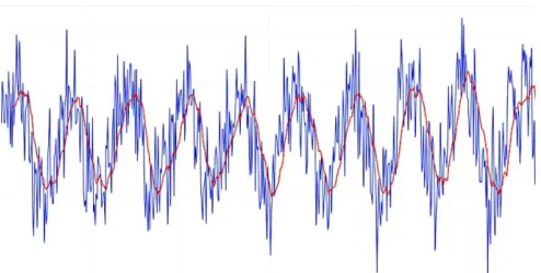
Fig. 1: Noisy Data (blue) and Data without noise (red)

The MFNR algorithm was simple in approach, much more powerful, with no need to tune the parameters, while light enough on resources, and was scalable to any desired error level.

Though MFNR algorithm was compared with standard image noise removal in three dimensional RGB images, but it can be extended to multi-dimensional data of all PDF types or even periodic type of data. For example, it can be used for noise removal in audio data.

II. RELATEDWORK

Presently, single frame noise removal method is standard and industry. Multi-frame Noise Removal is only a niche product [7]. The idea for MFNR is inspired from [7] which uses it to remove Gaussian Noise. Herein in this paper, the idea is generalized to include non-gaussian noise of all types, and of all dimensions. In this paper, we will be comparing several standard algorithms against MFNR including but not limited to NLM (Non-local Means), Median, Convolution Neural Networks.

NLM is one of the most effective noise removal tools for the Gaussian Noise. It has been shown that it performs better than other noise removal tools for the Gaussian noise [12]. Unlike other local-mean filters, which only take the surrounding pixels of the targeted pixel, NLM takes into account all the pixels thus having greater information at hand. This results in much more preservation of details [12].

But NLM still leaves ”method noise” in the process, which is more like ”white noise” [13]. Our proposed MFNR Algo-rithm doesn’t leave such noise because it is only estimating the same pixel and doesn’t take into account the surrounding pixels. MFNR algorithm can be extended to other image

Such pre-processing helps improve the results of the systems. Median filters are also very useful in signal processing.

Median filter works by taking the median value of the neighbouring data or pixels. Thus, we are essentially taking the ”window” which we slide in each step to ensure all of the pixels are taken care of. It works on multi-dimensional data. For 1-D, it simply works by taking into consideration the surrounding two values. Similar goes for more dimensional data.

Finally, MFNR is compared against Convolutional Autoen-coders for Image Noise removal [17] AutoenAutoen-coders have widely used for image noise reduction. Convolutional Net-works are the best known way to deal with images, frequently called CNN - Convolutional Neural Networks - or ConvNet. MFNR was found to be better in terms of Peak Signal to Noise Ratio (PSNR) than CNN.

III. PROPOSEDMETHOD

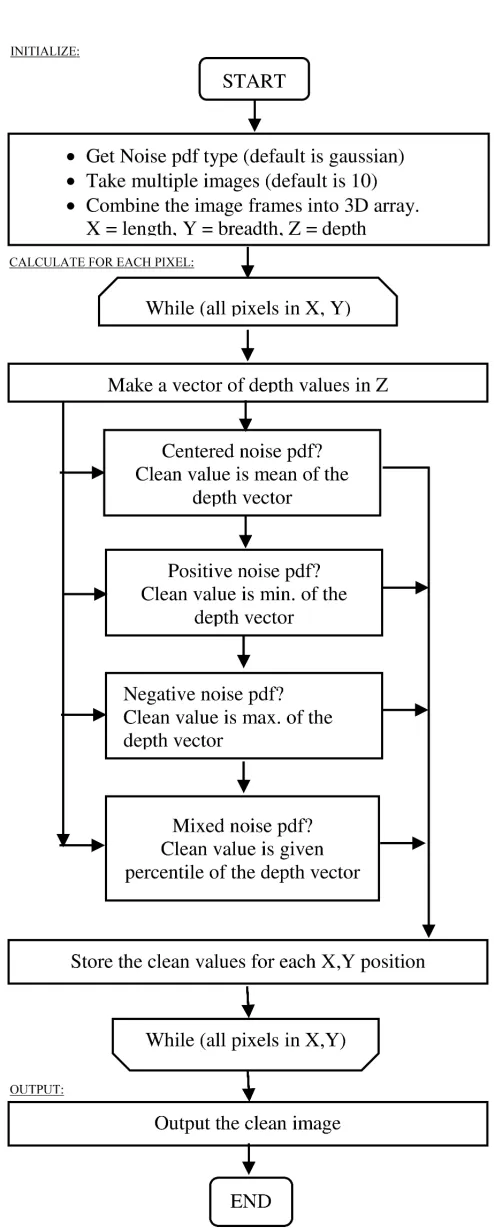
When an image is taken from a camera or any imaging sensor, noise is added to it, but because it is corrupted by “deterministic” noise, hence can be cleaned. It can be done only if the PDF (probability density function) of the noise is available, thus the information can be extracted against zero noise [6]. MFNR algorithm needs to know the type of noise involved to estimate and subsequently remove it. Its generalized form is depicted in Algorithm 1

Data:Collect multiple frames of the same data

while not all points of the data are processeddo

Load the similar position of data in each frame into an input array;

Apply MFNR Algorithm according to noise type, with that input array to predict the output; Store that output for the same position data

end

Result:Output the clean data

Algorithm 1: MFNR Generalized Algorithm

Fig. 2 shows the operational flow of MFNR algorithm as a specialized case for 3D RGB images. It takes multiple images, estimates the true value of the pixel given the noise type, and outputs the clean image. The algorithm is provided with the noise PDF type, and the number of images taken. The images are combined to make a 3D stack. X and Y axes denotes the length and breadth of images, while Z denotes the number of images or depth of the image stack. Pixels are traversed in all possible X,Y pairs, and for each pixel “depth vector” is defined containing the depth values. The “depth vector” estimates the noise, removes it for each depth vector, and corrects the corresponding pixel values. This provides a noise-free corrected image.

(a) (b)

(c) (d)

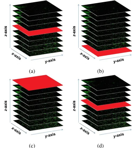
Fig. 3: Four types of Noise PDFs. (a) Centered Noise. (b) Positive Noise. (c) Negative Noise. (d) Mixed Noise

There are 4 PDF types on the large as shown in Fig. 3, i.e. Centered, Positive, Negative and Mixed noise PDF. Centered noise PDF has zero mean, e.g. Gaussian noise, salt & pepper noise and speckle noise. Positive noise PDF has all its values as positive, e.g. Gamma, Rayleigh, Poisson, exponential noise PDF’s. Negative noise PDF has all its values as negative, e.g. a uniform distribution with only negative values. Mixed noise PDF has some of the noise values lie on negative, and some on the positive side. Thus, its percentile needs to be obtained. We obtained it using the KDE algorithm. KDE can be applied in all four cases, but it is only really required in the mixed noise type. Types other than mixed noise can be cleaned simply by taking mean, max, min values. In cases where computational power is limited, mixed noise can be approximated with mean and we can still get pretty good results within required accuracy. For example, centered noise PDF is the special case of mixed PDF with 50% percentile. When mixed noise is added to the image, its minimum and maximum sample values need to be found. The percentile is the value corresponding to zero noise relative to the minimum and the maximum value. This value is found in a monte-carlo fashion.

How the noise is removed is shown in Fig. 4. Multiple frames of same image are taken at same resolution and in same position. They are aligned together, and given the noise PDF (Probability Density Function), its features are extracted for each pixel position through machine learning techniques for PDF detection. Multiple-images noise removal techniques have been used widely [6]. and its most common use is in astronomy, where low lightning condition is a limitation [7]. These techniques are mostly for Gaussian noise. The proposed algorithm is a generalized image noise removal tool catering for different noise types. It needs to know the type of noise involved, to estimate and remove it. For example, if the noise is Gaussian distributed, the MFNR algorithm is used to estimate the noise parameters from multiple images, and outputs the Gaussian mean as the corrected value for corresponding pixel values. However, if the noise is logarithmic or exponential, then MFNR algorithm needs to be adapted, accordingly.

(a) (b)

(c) (d)

Fig. 4: Four types of Noise PDFs and their noise cleaning Method. (a) Mean for Centered Noise. (b) Min for Positive Noise. (c) Max for Negative Noise. (d) Kernel Density Esti-mation (KDE) Mean for Mixed Noise

MFNR algorithm is simple to implement and the PSNR (Peak-Signal-to-Noise Ratio) improves as the number of frames are increased, and thus zero noise can be achieved. PSNR is defined as in Eqn. 1

PSNR= 10 log10

(2d₋₁₎2_{W H}

PW

i=1

PH

j=1(p[i, j]−p0[i, j])2 (1)

IV. EXPERIMENTALSETUP

The results were generated using Jupyter running Python on Windows x64 system. All the noise was simulated using standard libraries or otherwise explicitly mentioned.

V. PERFORMANCEEVALUATION A. Performance Measurements

As already discussed, MFNR algorithm is simple to imple-ment and the PSNR (Peak-Signal-to-Noise Ratio) improves as the number of frames are increased, and thus zero noise can be achieved. PSNR is defined as in Eqn. 2

PSNR= 10 log₁₀ (2

d₋₁₎2_{W H}

PW

i=1

PH

j=1(p[i, j]−p0[i, j])2 (2)

and thus compromising the fine details of the image. In general, a Gaussian filter is normally regarded as an “optimal” compromise and a default choice. There are other algorithms that may do better than Gaussian filters, but they are usually either too complex or require detailed knowledge of the noise form or structure that is not normally available, and can also require excessive computational power.

Multiple images are required for processing MFNR algo-rithm [8], and more the images better the noise removal. In short, number of images depends on the accuracy that needs to be achieved. The algorithm has numerous features making it preferable over other noise removal tools. Problem with other image noise removal algorithms is that, their parameters are often unknown most of the time, and frequently need to be estimated. For example, for applying NLM filter, patch size, window size, and noise level has to be given. It performs far better than even “optimal” filters like Gaussian, or Wiener Filter, and other complex filters.

When an image is taken from a camera or any imaging sensor, noise is added to it. The MFNR algorithm is simple to implement and the Peak Signal-to-Noise Ratio (PSNR) of the image improves as the number of frames are increased. [9] Multiple frames of same image are taken at same resolution and position. They are aligned, and given the noise Probability Density Function (PDF), its features are extracted for each pixel position.

Such multiple-images noise removal techniques have been used widely and its most common use is in astronomy, where low lightning condition is a limitation [7]. These techniques are mostly for gaussian noise. The proposed algorithm is a generalized image noise removal tool catering for different noise types.

In particular, it needs to know the type of noise involved, to estimate and then remove it. For example, if the noise is Gaussian distributed, the MFNR algorithm is used to estimate the noise parameters from multiple images, and outputs the gaussian mean as the corrected value for corresponding pixel values. However, if the noise is logarithmic or exponential, then MFNR algorithm uses KDE to find mean, accordingly [2].

There are a few basic PDF types considered here, specif-ically, Centered, Positive, Negative and Mixed noise PDF [4]. Centered noise PDF has zero mean, e.g. gaussian noise. Positive noise e.g. salt noise, and negative noise e.g. & pepper noise. Negative noise PDF has all its values as negative. Mixed noise examples include speckle noise, Gamma, Rayleigh, Poisson, exponential noise PDF’s. Mixed noise PDF has some of the noise values lie on negative, and some on the positive side. Thus, its percentile needs to be obtained using KDE. For example, centered noise PDF is the special case of mixed PDF with 50% percentile. When mixed noise is added to an image, its minimum and maximum sample values need to be found.

be done in real time in most modest applications. Generally, the requirements of MFNR algorithm are similar to those of Gaussian or Median filter, but actual time requirement depends on the implementation and optimization. Because it can remove most kinds of noise given the noise PDF, its application list is vast including cameras, ultrasound, PET, and MRI scan, or any other related application [11]. This algo-rithm can be successfully applied in the fields like medicine, RADAR, astronomy, with performance better than existing noise removal tools. In low light conditions, Gaussian noise is more profound, and MFNR algorithm can be the only solution. For example, cinema experience would be more enjoyable, if the video frames would be using MFNR algorithm to make crisp and sharp images especially during darker conditions. In addition, custom noise can also be removed, while most other filters are limited to fixed noise type.

This algorithm also has its share of limitations, such as being not able to remove hot pixels, and the inherent condition that multiple images are required. Also that, noise type must be known prior to processing.

The algorithm is versatile and the authors opine that this can be applied for removing the frequency domain noise also including the periodic noise where same signal which is peri-odic can make a PDF of its own and hence the deterministic signal can be extracted from the noise.

C. Performance Results

Performance against the Centered, Positive, Negative, and Mixed Noise removal were compared. Case studies were carried out comparing the performance of various filters in-cluding Gaussian, NLM, Median, Wiener, Neural, and MFNR for removing gaussian noise, using python, and the results compared. Similarly, salt and pepper noise and Poisson noise removal were also shown. Results are summarized in Fig. 5 showing the image noise removal comparison between different filters using simulated noise.

1) Centered Noise Removal [Gaussian Noise]: A sample image was taken and Gaussian noise was added to it. Then the noisy images were pre-processed with a number of different standard filters to remove the Gaussian noise [9]. Previously, Gaussian filter gave the maximum performance, but MFNR algorithm showed far greater PSNR performance. It was estimated that as the number of images were increased, the noise was removed in an exponential manner. The accuracy can be scaled according to requirements. Gaussian Filter is normally regarded as an “optimal” compromise and a default choice . There are other algorithms which may do better than Gaussian Filter, but they are usually either too complex or require lots of computational power.

(a)

(b)

(c)

(d)

Fig. 5: Four types of Noise PDFs and comparison of MFNR against standard algorithms (a) Centered Noise Removal [Gaussian Noise] (b) Positive Noise Removal [Salt Noise]. (c) Negative Noise Removal[Pepper Noise. (d) Mixed Noise Removal[Poisson Noise]

ρ(x) = 1

σ√2π exp

−(x−µ) 2

2σ2

,

F(x) = 1

σ√2π Z x

−∞

exp

−(t−µ) 2

2σ2

dt

(3)

2) Positive Noise Removal [Salt Noise]: Positive Noise such as a Salt noise [5] was removed and performance of different filters was compared. This result was more dramatic than previous MFNR (Gaussian) case with respect to the number of images used.

MFNR algorithm implies taking the minimum of the 10 samples, to reduce the noise. In this example, the actual value of the pixel was 0, but due to addition of salt noise, it was added in positive direction. After the application of MFNR algorithm, the actual value is restored to original value, so the noise was successfully removed. Eqn 4 depicts Salt Noise.

P(x) =

(

Pa,for x = a

0,otherwise (4)

3) Negative Noise Removal [Pepper Noise]: [5]

Similar to Salt noise. Pepper noise is removed by taking the largest value among the multiple frames for each pixel. Pepper noise is depicted in Eqn. 5

P(x) =

(

Pb,for x = b

0,otherwise (5)

4) Mixed Noise Removal [Poisson Noise]: The fundamental problem of density estimation is that of inferring the density functionf, given an i.i.d samplex1, x2, ..., xn from the corre-sponding probability distribution. The kernel density estimate (KDE) [2] is a particularly simple instance-based method. The idea is to compute the density of a test point as the average of the density of test point under each point in the training data. The estimate is given as in Eqn. 6

ˆ

f(x) = 1

nhd n

X

i=1

k _x−x

i

h

KDE maybe written as a linear system as in Eqn. 8,

ˆ

f(x) =Kw, (8)

where

wi=

1

nkij=

1

hdk

_x

−xi

h

. (9)

Thus, we can see that w makes the convex combination. Any alterations to K will have corresponding results.

Herein, the log-likelihood estimate of any given sample is depicted as in Eqn. 10

L(x) = 1

n X

i

log ˆf(xi)

L(x) = 1

n X i log 1 nhd n X j=1 k _x

i−xj2

h

.

(10)

And its differential is given as in Eqn. 11,

∂L ∂xi = 1 nh2 X j

exp−||xi−yj||2

2h2

P

kexp

−||xi−yk||2

2h2

(yj−xi), (11)

It can be shown that xi is moving towards the center yj proportional to its weightage whereby xi is toyj.

The gradiant of the log-likelihood w.r.t. centers yj is as shown in Eqn. 12

∂L ∂yj = 1 nh2 X i

exp−||xi−yj||2

2h2

P

kexp

−||xi−yk||2

2h2

(xi−yj), (12)

where yj moves to the points xi in step to how close xi already is to yj.

The gradiant of the estimate of the resubstitution entropy is as shown in Eqn. 13

∂h

∂x =−

_∂L

∂x;+

∂L ∂;x

, (13)

herein x; and;xare the first and second arguments of L, respectively.

The gradiant of the KL divergence estimate is given as in Eqn. 14,

∂D

∂x =

_∂L(x;x)

∂x; +

∂L(x;x)

∂;x

−∂L(x;y)

∂x ∂D

∂y =−

∂L(x;y)

∂y .

(14)

The histogram density with bin widthhis as shown in Eqn. 15

f(x) = 1

nh(number of xi in same bin asx). (15)

f(x) = 1

n X

i

K(x, xi)

= 1

n X

i

φ(x)0φ(xi)

=φ(x)01

n X

i

φ(xi).

(16)

So the implicit training in a KDE is simply taking an average.

Herein, we applied KDE on the Poisson distribution. [3] The shorthand X ∼ Poisson(µ) is the indicator of random variable X and that it has the distribution of the Poisson wherein the positive parameter is µ. The random variable X

having scale parameterµhas the probability mass function as showin in Eqn. 17

f(x) =µ

x_e−µ

x! x= 0,1,2, . . . . (17)

The number of events can be modelled by the Poisson in an interval associated over the space or time with random variables. For example, the number of potholes over a road, or the number of typographical errors in a magazine, or the frequency of the descent of customers per hour, or the number of earthquakes in a decade. It can also approximate the binomial distribution whereinnis very large andpis very small.

VI. CONCLUSION& FUTUREWORKS

It was shown that our proposed MFNR algorithm performed much better at noise removal than conventional noise removal tools. Their performance was compared at the removal of Gaussian, Salt and Pepper, and Poisson noise as special case of MFNR Algorithm applied to 3D data of colored images. General MFNR Algorithm can be extended to multi-dimensional data of all types of noises. The PSNR was used as a performance metric. Due to its logarithmic nature, even a sin-gle point is worth it, but we were able to achieve significantly beyond that. In fact, MFNR Algorithm can practically remove the noise completely. More frames require more availability of frames and computational power, hence the algorithm can be tailored to individual needs. The algorithm can also be applied to remove the periodic noises. It is proposed that this newer approach should be used to improve upon existing medical, defence, astronomy, and numerous fields where performance needs to be enhanced which is currently limited by noisy data which is difficult to remove.

REFERENCES

[1] J. Scharcanski and A. N. Venetsanopoulos, ”Edge detection of color images using directional operators,” Circuits and Systems for Video Technology, IEEE Transactions on, vol. 7, pp. 397-401, 1997. [2] Varet, Suzanne, et al. ”Numerical performance of Penalized

Compar-ison to Overfitting for multivariate kernel density estimation.” arXiv preprint arXiv:1902.01075 (2019).

[3] Lizama, Carlos. ”The Poisson distribution, abstract fractional difference equations, and stability.” Proceedings of the American Mathematical Society 145.9 (2017): 3809-3827.

[4] Razak, Alina, et al. ”Talker identification in three types of background noise.” The Journal of the Acoustical Society of America 141.5 (2017): 4039-4039.

[5] Varatharajan, R., et al. ”An adaptive decision based kriging interpola-tion algorithm for the removal of high density salt and pepper noise in images.” Computers & Electrical Engineering 70 (2018): 447-461. [6] A. Buades, Y. Lou, J.-M. Morel, and Z. Tang, ”Multi image noise

estimation and denoising,” preprint, Aug, 2010.

[7] S. D. Gwyn, ”MegaPipe: The MegaCam image stacking pipeline at the Canadian astronomical data centre,” Publications of the Astronomical Society of the Pacific, vol. 120, pp. 212-223, 2008.

[8] Farsiu, Sina, Michael Elad, and Peyman Milanfar. ”Multiframe demo-saicing and super-resolution of color images.” IEEE transactions on image processing 15.1 (2005): 141-159.

[9] Li, Xuelong, et al. ”A multi-frame image super-resolution method.” Signal Processing 90.2 (2010): 405-414.

[10] Van Noort, Michiel, Luc Rouppe Van Der Voort, and Mats G. L¨ofdahl. ”Solar image restoration by use of multi-frame blind de-convolution with multiple objects and phase diversity.” Solar Physics 228.1-2 (2005): 191-215.

[11] Liu, Yuncai, and Thomas S. Huang. ”Vehicle-type motion estimation from multi-frame images.” IEEE Transactions on Pattern Analysis and Machine Intelligence 15.8 (1993): 802-808.

[12] Buades, Antoni (20–25 June 2005). A non-local algorithm for image denoising. Computer Vision and Pattern Recognition, 2005. 2. pp. 60–65. CiteSeerX 10.1.1.103.9157. doi:10.1109/CVPR.2005.38. ISBN 978-0-7695-2372-9.

[13] Dehghannasiri, R.; Shirani, S. (2012). ”A novel de-interlacing method based on locally-adaptive Nonlocal-means”. 2012 Con-ference Record of the Forty Sixth Asilomar Conference on Signals, Systems and Computers (ASILOMAR). pp. 1708–1712. doi:10.1109/ACSSC.2012.6489324. ISBN 978-1-4673-5051-8. [14] Dehghannasiri, R.; Shirani, S. (2013). ”A view interpolation method

without explicit disparity estimation”. 2013 IEEE International Con-ference on Multimedia and Expo Workshops (ICMEW). pp. 1–4. doi:10.1109/ICMEW.2013.6618274. ISBN 978-1-4799-1604-7. [15] Martinello, Manuel; Favaro, Paolo. ”Depth Estimation From a Video

Sequence with Moving and Deformable Objects” (PDF). IET Image Processing Conference.

[16] Huang, Thomas S.; Yang, George J.; Tang, Gregory Y. (February 1979). ”A fast two-dimensional median filtering algorithm” (PDF). IEEE Transactions on Acoustics, Speech, and Signal Processing. 27 (1): 13–18. doi:10.1109/TASSP.1979.1163188.

[17] Gondara, Lovedeep. ”Medical image denoising using convolutional denoising autoencoders.” 2016 IEEE 16th International Conference on Data Mining Workshops (ICDMW). IEEE, 2016.

Awais Nazir received his Bachelor’s degree in Electrical Engineering from National University of Sciences and Technology (Islamabad, Pakistan) in 2012, and Master’s degree from National University of Sciences and Technology in Electrical Engineer-ing in 2015. He has diverse industrial and academia experience in his field as Project Manager at various Engineering and Research Projects. Currently he is pursuing his PhD in Electrical Engineering from Na-tional University of Sciences. His research interests include Data Science, Artificial Intelligence, Bio-Medical Engineering, and Computer Vision.

Muhammad Shahzad Younisreceived the bache-lor’s degree from National University of Sciences and Technology, Islamabad, Pakistan, in 2002, the master’s degree from the University of Engineer-ing and Technology, Taxila, Pakistan, in 2005, and the PhD degree from University Technology PETRONAS, Perak, Malaysia in 2009, respectively. Before joining National University of Sciences and Technical (NUST), he was Assistant Manager at a research and development organization named AERO where he worked on different signal pro-cessing and embedded system design applications. He is currently working as an Assistant professor in the Department of Electrical Engineering in School of Electrical Engineering and Computer Science (SEECS)-NUST. He has published more than 25 papers in domestic and international journals and conferences. His research interests include Statistical Signal Processing, Adaptive Filters, Convex Optimization Biomedical signal processing, wireless communication modelling and digital signal processing.