Tight Reductions for Diffie-Hellman Variants in the Algebraic Group Model

Tight Reductions for Diffie-Hellman Variants in the

Algebraic Group Model

Taiga Mizuide†, Atsushi Takayasu‡, Tsuyoshi Takagi§

June 29, 2019

Abstract

Fuchsbauer, Kiltz, and Loss (Crypto’18) gave a simple and clean definition of an alge-braic group model (AGM) that lies in between the standard model and the generic group model (GGM). Specifically, an algebraic adversary is able to exploit group-specific structures as the standard model while the AGM successfully provides meaningful hardness results as the GGM. As an application of the AGM, they showed a tight computational equivalence between the computing Diffie-Hellman (CDH) assumption and the discrete logarithm (DL) assumption. For the purpose, they used the square Diffie-Hellman assumption as a bridge, i.e., they first proved the equivalence between the DL assumption and the square Diffie-Hellman assumption in the AGM, then used the known equivalence between the square Diffie-Hellman assumption and the CDH assumption in the standard model. In this paper, we provide an alternative proof that directly shows the tight equivalence between the DL assumption and the CDH assumption. The crucial benefit of the direct reduction is that we can easily extend the approach to several variants of the CDH assumption, e.g., the bilinear Diffie-Hellman assumption. Indeed, we show several tight computational equivalences and discuss applicabilities of our techniques. In this full version, we provide further applications (including thematrix computational Diffie-Hellman assumption and thekernel matrix Diffie-Hellman assumption) and a detailed overview of our techniques.

∗_{We would like to thank anonymous reviewers of CT-RSA 2019 for their helpful comments and suggestions. This}

research was supported by JST CREST Grant Number JPMJCR14D6, Japan. This is the full version of [MTT19]. †_{Department of Creative Informatics, The University of Tokyo.}

‡_{Department of Mathematical Informatics, The University of Tokyo and National Institute of Advanced Industrial}

Contents

1 Introduction 3

1.1 Background . . . 3

1.2 Our Contributions . . . 4

1.3 Technical Overview . . . 5

1.4 Organization . . . 6

2 Computational Problems 6 2.1 Diffie-Hellman Variants in Cyclic Groups . . . 6

2.2 Diffie-Hellman Variants in Symmetric Bilinear Groups . . . 7

2.3 Matrix Diffie-Hellman Problem . . . 8

3 Algebraic Group Model 11 4 Reductions for Diffie-Hellman Variants in Cyclic Groups 13 4.1 DL to CDH Reduction via Affine Embedding . . . 13

4.2 Master Theorem in Cyclic Groups . . . 14

5 Reductions for Diffie-Hellman Variants in Symmetric Bilinear Groups 16 5.1 Algebraic Symmetric Bilinear Group Model . . . 16

5.2 BDL to CBDH Reduction via Affine Embedding . . . 16

5.3 Master Theorem in Symmetric Bilinear Groups . . . 18

6 Reduction for Matrix Computational Diffie-Hellman Problem 20 6.1 Algebraic Group Model for Matrix Computational Diffie-Hellman Problem. . . 21

6.2 BDL to Computational k-Lin Reduction via Implicit Embedding . . . 21

6.3 Master Theorem for Matrix Computational Diffie-Hellman Problem . . . 22

7 Reduction for Matrix Kernel Diffie-Hellman Problem 26 7.1 Algebraic Group Model for Matrix Kernel Diffie-Hellman Problem . . . 27

7.2 Master Theorem for Matrix Kernel Diffie-Hellman Problem . . . 27

1

Introduction

1.1 Background

Diffie-Hellman Problem in the Generic Group Model. The discrete logarithm (DL) as-sumption and the computational Diffie-Hellman (CDH) asas-sumption including its variants have been devoted to constructing numerous cryptographic protocols. Hence, estimating the computational hardness of solving the problems is a fundamental research topic in cryptography. For the pur-pose, thegeneric group model (GGM) [Nec94,BL96,Sho97,MW98,Mau05] over cyclic groups is a wonderful tool and has successfully provided several fantastic results in the context. Generic al-gorithms are not able to exploit specific structures of cyclic groups in the sense that the alal-gorithms are given group elements only via abstract handles. Then, the algorithms are able to output only group elements which are computed by interacting with an oracle and applying group operations to given elements. Therefore, generic algorithms such as a baby-step giant-step algorithm, the Pohlig-Hellman algorithm [PH78] (in composite-order groups), and Pollard’s rho algorithm [Pol78] work in any cyclic groups.

Furthermore, the most substantial benefit of the GGM is that we are able to derive information theoretic lower bounds of computational problems, where analogous analyses seem infeasible in the standard model. For example, any generic algorithms require at least O(√p) group operations to solve the DL problem in cyclic groups of a prime-orderp. Analogous analyses have also been made for the CDH problem and its variants in an ad-hoc manner. Thus far, the GGM has been extended and used for studying computational problems in bilinear (and multilinear) groups [BB08,Boy08, KSW13,MRV16,EHK+17].

One main criticism of the GGM is that computational problems that are generically hard may not be hard when instantiated in concrete groups. Jager and Schwenk [JS13] proved that computing a Jacobi symbol of an integer modulo a composite n generically is equivalent to factorization; however, the computation is easy when given an actual representation ofZn. Similarly, the number field sieves [Gor93] in specific groups are able to solve the DL problem in subexponential time in logp, i.e., faster than the generic algorithms. Hence, the GGM gives us certain confidence of computational hardness while we want to obtain analogous results in the standard model or less restricted models than the GGM.

Algebraic Group Model. In Crypto’18, Fuchsbauer, Kiltz, and Loss [FKL18] introduced an algebraic group model (AGM). The definition of the AGM lies in between the standard model and the GGM. Like the standard model and unlike the GGM, an algebraic algorithm is given an actual representation of cyclic groups. On the other hand, like the GGM and unlike the standard model, an algebraic algorithm is able to output only group elements by applying group operations to given elements. Although the algebraic algorithm is not required to interact with an oracle for the compu-tation, it should output a record of a group operation which Fuchsbauer et al. called a representa-tion. LetG:= (G, G, p) be a group description, whereGis an additive cyclic group of a prime-order

p and G is a generator. When an algebraic algorithm is given

(

G, ⃗X := (X1, . . . , Xℓ)∈Gℓ

)

and

outputsZ ∈G, it has to also output a vector⃗z:= (z0, z1, . . . , zℓ)∈Zℓp+1 as a representation of Z with respect to X⃗ such that Z =∑ℓ_i=0ziXi, where X0 := G. Similar definitions of an algebraic algorithm are already known in [BV98, PV05]; however, Fuchsbauer et al.’s definition is simpler and clearer.

problem [MW96,BDS98] as an intermediate step. They first proved a tight reduction from the DL to the square DH in the AGM. Let (G, X) be a DL instance such that X := xG. The reduction algorithm gives (G, X) to a square DH algorithm and receives an answer Z = x2G along with a representation vector⃗z. Fuchsbauer et al. showed that the vector⃗z and the relation

z0G+z1X=Z

are sufficient to recover the DL solutionxby solving an equation modulo a primep. Then, thanks to the known computational equivalence between the square DH and the CDH [MW99,BDZ03], their reduction implies a tight reduction from the DL to the CDH in the AGM. Furthermore, a valuable feature of the result is that the reduction algorithm isgeneric. Due to the fact, an existence of the tight reduction implies an information theoretic lower bounds of the CDH asO(√p) in the GGM. Fuchsbauer et al. claimed that a benefit of the AGM is that we are able to derive information theoretic lower bounds of the CDH in the GGM via quite simple arguments. Indeed, Fuchsbauer et al.’s reduction in the AGM is much simpler than the analogous analysis in the GGM. Therefore, providing generic reductions from the DL to other computational problems of the CDH family in the AGM has to be an interesting open problem.

1.2 Our Contributions

In this paper, we provide generic and tight reductions from the DL to several computational prob-lems of the CDH family in the AGM. A starting point of our technique is adirect reduction from the DL to the CDH without using the square DH as the intermediate step. Given the DL in-stance (G, X), our reduction algorithm randomly samplesr∈Zp and gives (G,(X1, X2)) to a CDH

algorithm, where

X1 :=X=xG and X2 :=X+rG= (x+r)G.

Here, (G,(X1, X2)) is a properly distributed CDH instance in the sense that x and x+r are independently distributed to uniform inZp from the CDH algorithm’s view. Then, the reduction algorithm receives a solution of the CDHZ =x(x+r)Galong with a representation vector⃗z. We show that the vector⃗z and the relation

z0G+z1X1+z2X2 =Z

are sufficient to recover x by solving an equation modulo a primep. The approach is very simple as Fuchsbauer et al.’s one and easily applicable to several CDH variants which are not studied in [FKL18]. We believe that the simplicity is a main benefit of our result. To explain our technique as simple as possible, we consider only tight reductions in the sense that the reduction algorithm uses an algorithm for CDH variantsonly once.

Furthermore, we extend the AGM to an algebraic bilinear group model (ABGM) for studying computational problems in symmetric bilinear groups equipped with a mape:G×G→GT. We define an algebraic bilinear algorithm so that it is given(G:= (G,GT, G, e, p), ⃗X := (X1, . . . , Xk)∈

Gk_{, ⃗Y := (Y1, . . . , Y}

ℓ)∈Gℓ_T

)

and outputsZ ∈GT along with a representation vector⃗zthat indicates howZ is computed by the given elements. Then, we extend the approach used in cyclic groups and provide generic and tight reductions from the DL to several computational problems of the CDH family including the computational bilinear Diffie-Hellman problem.

In the preliminary version [MTT19], our master theorem in cyclic groups does not capture the computational k-linear problem. Thus, we gave a tailor-made reduction for the problem. In this full version, we provide a new master theorem for the matrix computational Diffie-Hellman problem that includes the computational k-linear problem as a special case. Furthermore, we show a new application called the kernel matrix Diffie-Hellman problem in this full version.

1.3 Technical Overview

In this subsection, we provide more detailed explanation of our technique, where the discussion did not appear in the preliminary version [MTT19].

In [FKL18], the reduction algorithm of Fuchsbauer et al. gives (G, X), which is exactly the DL instance, to a square DH algorithm. We call the reduction approach an identity embedding since the DL solution x is used only by xG = X as a group element. In other words, even if we want to use an algorithm which takes multiple group elements (X1, X2, . . .) as the input, the identity embedding can embed the DL solution x into only one group element. Since the square DH is computationally equivalent to the CDH in the standard model, the identity embedding is enable to show a computational equivalence between the DL and the CDH by using the square DH as the intermediate bridge.

However, the identity embedding looks insufficient for providing a direct reduction from the DL to the CDH. The limitation of the identity embedding is that the DL solution is used only for one group element. When we try to use the identity embedding to provide a reduction for the CDH, the reduction algorithm randomly samples r∈Zp and sets

X1 :=X =xG and X2 :=rG.

However, in this case the relation

z0G+z1X1+z2X2 =Z

obtained by the output of the CDH algorithm is insufficient for recovering the DL solution x. Intuitively, the output of the CDH algorithm xrG does not give the reduction algorithm any additional information, since the reduction algorithm is able to compute Z=xrG=rX by itself.

To this end, we introduce a new embedding which we call anaffine embedding. As claimed above, when we provide a reduction for the CDH problem, the reduction algorithm gives (G,(X1, X2)) to

a CDH algorithm, where

X1 :=X=xG and X2 :=X+rG= (x+r)G

by picking a random r ∈ Zp. The affine embedding embeds the DL solution x into two group elements (X1, X2), where x +r that is an exponent of X2 has an affine relation of x. Then, the reduction algorithm is able to obtain non-trivial information since it is not able to compute

Z =x(x+r)G(orx2G) by itself. Similarly, the affine embedding is able to embed the DL solution

x into multiple group elements ((x+r1)G, . . . ,(x+rℓ)G) by picking random (r1, . . . , rℓ) ∈ Zℓp. Note that the discrete logarithm of group elements (x, x+r1, . . . , x+rℓ) look random inZℓp+1 from Diffie-Hellman algorithm’s view.

The affine embedding is still insufficient for the computational k-linear problem, i.e., given (G, X1 := x1G, . . . , Xk := xkG, Y1 := x1y1, . . . , Yk := xkykG) for random (x1, . . . , xk, y1, . . . , yk) and compute (y1 +· · ·+yk)G. Specifically, by embedding an affine relation of the DL solution

may result in a zero polynomial. To avoid the obstacle, we sample a random x1 by ourselves and

implicitly embed the DL solutionx intox1y1. We call the embedding implicit embedding since we

do not know a value of y1. In other words, a k-linear algorithm enables us to obtain a non-trivial valuey1 =x1/xthat enables us to provide a reduction from the DL to thek-linear problem.

1.4 Organization

In Section2, we review several computational problems which we study in this paper. In Section3, we review a definition of the algebraic group model (AGM) defined by Fuchsbauer et al. [FKL18]. In Sections 4 and 5, we show our technique to provide generic and tight reductions from the DL to the CDH family in cyclic groups and symmetric bilinear groups along with master theorems, respectively. In Sections 6 and 7, we show new applications of this full version, i.e., generic and tight reductions from the DL problem to the matrix computational Diffie-Hellman problem and the matrix kernel Diffie-Hellman problem, respectively.

Notations. We usex←$ Zp to denote a uniformly random sampling fromZpand (x1, . . . , xℓ)

$

←Zℓ p to denote every element is sampled by xi

$

← Zp independently. Let a capital case bold letter A and a lower case bold letter adenote a matrix and a column vector, respectively. Let0k denote a

k-dimensional zero vector. For an (m+n)-variate polynomialf(x1, . . . , xm, y1, . . . , yn), we use degf to denote a degree of the polynomial and deg_x1,...,xmf to denote a degree of the polynomial only with respect to variables x1, . . . , xm. As an example for f(x, y, z) := x2yz, we use the notations degf = 4, deg_xf = 2, and deg_x,y = 3. As a notational convenience, we use degf = 1/k for

f =x1/k and degf =−k forf =x−k.

2

Computational Problems

In this section, we review several computational problems that we study in this paper. Specifically, in Sections 2.1, 2.2, and 2.3, we review Diffie-Hellman variants in cyclic groups, symmetric bilin-ear groups, and matrix Diffie-Hellman problems in asymmetric bilinbilin-ear groups, respectively. The contents of this section refer to [Boy08,KSW13,MRV16,EHK+17].

2.1 Diffie-Hellman Variants in Cyclic Groups

We review computational problems in cyclic groups. Let G := (G, G, p) be a group description, whereGis an additive group generated byGand has a prime-order p.1 For simplicity, when given

G we use the notation [a] :=aGfora∈Zp.

We first define a discrete logarithm problem to which other problems will be reduced.

Definition 1 (Discrete Logarithm (DL) Problem). Given a group description G := (G, G, p) and a group element X:= [x]∈G;x←$ Zp, compute x∈Zp.

Then, we summarize the CDH problem and its variants which we study in this paper.

Definition 2 (Computational Diffie-Hellman (CDH) Problem [DH76]). Given a group description

G := (G, G, p) and group elements (X1 := [x1], X2 := [x2]) ∈ G2; (x1, x2) ←$ Z2_p, compute Z := [x1x2]∈G.

1 _{To construct a reduction, we solve an equation modulo an order ofG. Hence, if the order is composite, we do}

Definition 3 (k-party Diffie-Hellman (k-PDH) Problem [Bis08]). Given a group description G := (G, G, p) and group elements (X1 := [x1], . . . , Xk := [xk]) ∈Gk; (x1, . . . , xk)

$ ← Zk

p, compute Z := [x1· · ·xk]∈G.

The followingk-exponent Diffie-Hellman assumption fork= 2 called the square Diffie-Hellman assumption was used in [MW96,BDS98].

Definition 4 (k-exponent Diffie-Hellman (k-EDH) Problem). Given a group description G := (G, G, p) and a group element X:= [x]∈G;x←$ Zp, compute Z := [xk]∈G.

The following k-th root Diffie-Hellman problem fork= 2 called the square root Diffie-Hellman problem was used in [KMS04].

Definition 5 (k-th Root Diffie-Hellman (k-RDH) Problem). Given a group description G := (G, G, p) and a group element X:= [x]∈G;x←$ Zp, compute Z := [x1/k]∈G.

The following k-Inverse Diffie-Hellman problem for k = 1 called the inverse computational Diffie-Hellman problem was used in [BDZ03].

Definition 6 (k-Inverse Diffie-Hellman (k-IDH) Problem). Given a group description G := (G, G, p) and a group element X:= [x]∈G;x←$ Zp, compute Z := [x−k]∈G.

To provide our master theorem in cyclic groups, we define a generalized version of the Diffie-Hellman problem as follows.

Definition 7 (Generalized Diffie-Hellman (GDH) Problem). Let f1(x1, . . . , xm, y1, . . . , yn), . . . ,

fℓ(x1, . . . , xm, y1, . . . , yn), and g(x1, . . . , xm) be known fixed non-zero polynomials. Given a group description G := (G, G, p) and group elements

(X1:= [f1(x1, . . . , xm, y1, . . . , yn)], . . . , Xℓ := [fℓ(x1, . . . , xm, y1, . . . , yn)])∈Gℓ; (x1, . . . , xm, y1, . . . , yn)

$ ←Zm+n

p ,

compute

Z := [g(x1, . . . , xm)]∈G.

Note that the GDH problem contains the CDH, the k-PDH, the k-EDH, thek-RDH, and the

k-IDH problem as special cases.

2.2 Diffie-Hellman Variants in Symmetric Bilinear Groups

We review computational problems in bilinear groups. For simplicity, we focus only onsymmetric bilinear mapse:G×G→ GT. Let G := (G,GT, G, e, p) be a bilinear group description, whereG is an additive group generated by Gand has a prime-order p, andGT is a multiplicative group of order passociated with a non-degenerate bilinear mape:G×G→GT, i.e., e(G, G) is a generator

ofGT and e(xG, yG) =e(G, G)xy. For simplicity, when givenGwe use the notations [a] :=aGand

[a]T :=e(G, G)a fora∈Zp.

We will provide a reduction from the DL in source groupsGto CDH variants. Hence, we define a bilinear discrete logarithm problem as follows.

Definition 8 (Bilinear Discrete Logarithm (BDL) Problem). Given a bilinear group description

G:= (G,GT, G, e, p) and a group elementX := [x]∈G;x

$

Then, we summarize the CDH variants in symmetric bilinear groups.

Definition 9 (Computational Bilinear Diffie-Hellman (CBDH) Problem [BF03,Jou04]). Given a bilinear group description G := (G,GT, G, e, p) and group elements (X1 := [x1], X2 := [x2], X3 :=

[x3])∈G3; (x1, x2, x3)

$ ←Z3

p, compute Z := [x1x2x3]T ∈GT.

Definition 10 (k-party Bilinear Diffie-Hellman (k-PBDH) Problem). Given a group description

G := (G,GT, G, e, p) and group elements (X1 := [x1], . . . , Xk := [xk]) ∈ Gk; (x1, . . . , xk)

$ ← Zk

p, computeZ := [x1· · ·xk]T ∈GT.

Definition 11(k-exponent Bilinear Diffie-Hellman (k-EBDH) Problem). Given a group description

G:= (G,GT, G, e, p) and a group elementX := [x]∈G;x

$

←Zp, compute Z := [xk]T ∈GT.

Definition 12(k-th Root Bilinear Diffie-Hellman (k-RBDH) Problem). Given a group description

G:= (G,GT, G, e, p) and a group elementX := [x]∈G;x

$

←Zp, compute Z := [x1/k]T ∈GT.

Definition 13 (k-Inverse Bilinear Diffie-Hellman (k-IBDH) Problem). Given a group description

G:= (G,GT, G, e, p) and a group elementX := [x]∈G;x

$

←Zp, compute Z := [x−k]T ∈GT.

To provide our master theorem in bilinear groups, we define a generalized version of the bilinear Diffie-Hellman problem as follows.

Definition 14 (Generalized Bilinear Diffie-Hellman (GBDH) Problem). Let f1(x1, . . . , xm, y1, . . . , yn), . . . , fk(x1, . . . , xm, y1, . . . , yn),g1(x1, . . . , xm, y1, . . . , yn), . . . , gℓ(x1, . . . , xm, y1, . . . , yn), and

h(x1, . . . , xm) be known fixed non-zero polynomials. Given a bilinear group description G :=

(G,GT, G, e, p) and group elements

(

X1 := [f1(x1, . . . , xm, y1, . . . , yn)], . . . , Xk:= [fk(x1, . . . , xm, y1, . . . , yn)],

Y1:= [g1(x1, . . . , xm, y1, . . . , yn)]T, . . . , Yℓ := [gℓ(x1, . . . , xm, y1, . . . , yn)]T

)

∈Gk_×Gℓ T;

(x1, . . . , xm, y1, . . . , yn)

$ ←Zm+n

p ,

compute

Z := [h(x1, . . . , xm)]T ∈GT.

Note that the GBDH problem contains the CBDH, the k-PBDH, the k-EBDH, the k-RBDH, and thek-IBDH problem as special cases.

2.3 Matrix Diffie-Hellman Problem

We review matrix Diffie-Hellman problems in asymmetric bilinear groups2. Let G := (G,GT,

G1, G2, e, p) be an asymmetric bilinear group description, where G1 and G2 are additive groups

generated by G1 and G2 respectively, and has a prime-order p, and GT is a multiplicative group of order p associated with a non-degenerate bilinear map e : G1 ×G2 → GT, i.e., e(G1, G2) is a

generator ofGT ande(xG1, yG2) =e(G1, G2)xy. For simplicity, when givenG we use the notations [a]1 :=aG1, [a]2 := aG2, and [a]T := e(G1, G2)a fora∈Zp. Furthermore, for a matrixA= (ai,j) we use the notation [A]1 to denote a matrix whose every (i, j) element is [ai,j]1. We use analogous

notations to denote [A]2 and [A]T.

Matrix Distribution. Let Dk be a matrix distribution to sample a matrix A ∈ Z(pk+1)×k. Let ¯

A and a⊤ denote a top k×k submatrix and a bottom row vector of A, respectively. Escala

2

et al. [EHK+17] introduced a matrix decisional Diffie-Hellman (matrix DDH) problem. Roughly speaking, the matrix DDH problem states that ([A]1,[As]1) and ([A]1,[u]1) in G(1k+1)×k×G

k+1 1

are computationally indistinguishable, whereA← Dk,s

$

←Zk

p, andu

$

←Zk+1

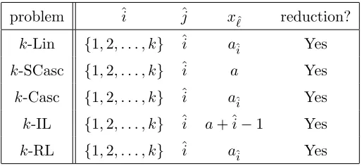
p . The matrix DDH contains several decisional problems as special cases. For example, we show examples of matrix distributions Dk for theSymmetric k-Cascade assumption (SCk), the k-Cascade assumption (Ck), the decisional k-linear assumption (Lk), the incremental k-linear assumption (ILk) that were introduced in [EHK+17], and the randomized k-linear assumption (RLk) that were introduced in [JR14] (they called the assumptionk-lifted assumption and the randomizedk-linear assumption was named in [MRV16]) as follows:

Lk:A=

     a1 0 . ..

0 ak

1 · · · 1

   

, SCk :A=

      a 0

1 . .. . .. a

0 1     

, Ck:A=       a1 0

1 . .. . .. ak

0 1      ,

ILk :A=

       a 0

a+ 1

. ..

0 a+k−1

1 · · · 1

      

, RLk:A=

    

a1 0

. ..

0 ak

ak+1 · · · a2k

    .

We define a generalized matrix distribution to provide our master theorems as follows:

Definition 15 (Generalized Matrix DistributionGMk). Let fi,j(x1, . . . , xm) be known fixed poly-nomials (which may include zero polypoly-nomials) for (i, j) ∈ {1,2, . . . , k+ 1} × {1,2, . . . , k}. The generalized matrix distribution GMk is defined by A= (ai,j)∈Z(pk+1)×k for

ai,j =fi,j(x1, . . . , xm); (x1, . . . , xm)

$ ←Zm

p ,

where

• _A¯ _{is full rank with overwhelming probability.}

• There is at least one indexj ∈ {1,2, . . . , k} such that fk+1,j(x1, . . . , xm)are non-zero polyno-mials.

We use the notation Xi,j to denote [ai,j]1.

We will provide generic and tight reductions for computational counter parts of matrix Diffie-Hellaman problems based on the following bilinear discrete logarithm problem in a group G1.

Definition 16 (Bilinear Discrete Logarithm (BDL) Problem in G1). Given a bilinear group

de-scription G := (G1,G2,GT, G1, G2, e, p) and a group element X := [x]1 ∈ G1;x

$

← Zp, compute

x∈Zp.

In this paper, we study computational counterparts of the matrix DDH assumption in the following two ways as [MRV16].

Matrix Computational Diffie-Hellman Problem. The first computational counterpart is the matrix computational Diffie-Hellman (MCDH) problem. Roughly speaking, the MCDH problem states that given ([A]1,[ ¯As]1) ∈G₁(k+1)×k×G₁k+1 then computing [a⊤s]1 ∈G1 is computationally

hard, whereA← Dk ands

$

Definition 17 (Computational k-Linear (k-Lin) Problem). Given a group description G := (G,GT, G1, G2, e, p) and group elements (X1 := [x1]1, . . . , Xk := [xk]1, Y1 := [x1y1]1, . . . , Yk := [xkyk]1)∈G12k+1; (x1, . . . , xk, y1, . . . , yk)

$ ←Z2k

p , compute Z := [y1+· · ·+yk]1 ∈G1.

Definition 18 (Computational Symmetric k-Cascade (k-SCasc) Problem). Given a group de-scription G := (G,GT, G1, G2, e, p) and group elements (X := [x]1, Y1 := [xy1]1, Y2 := [y1 + xy2]1, . . . , Yk:= [yk−1+xyk]1)∈Gk1+1; (x, y1, . . . , yk)

$ ←Zk+1

p , compute Z:= [yk]1 ∈G1.

Definition 19 (Computational k-Cascade (k-Casc) Problem). Given a group description G := (G,GT, G1, G2, e, p) and group elements (X1 := [x1]1, . . . , Xk := [xk]1, Y1 := [x1y1]1, Y2 := [y1+

x2y2]1, . . . , Yk:= [yk−1+xkyk]1)∈G21k; (x1, . . . , xk, y1, . . . , yk)

$ ←Z2k

p , compute Z := [yk]1∈G1.

Definition 20 (Computational Incrementalk-Linear (k-IL) Problem). Given a group description

G:= (G,GT, G1, G2, e, p) and group elements (X:= [x]1, Y1 := [x1y1]1, Y2 := [(x+ 1)y2]1, . . . , Yk:= [(x+k−1)yk]1)∈Gk1+1; (x, y1, . . . , yk)

$ ←Zk+1

p , compute Z:= [y1+· · ·+yk]1 ∈G1.

Definition 21 (Computational Radnomized k-Linear (k-RL) Problem). Given a group

descrip-tion G := (G,GT, G1, G2, e, p) and group elements (X1 := [x1]1, . . . , X2k := [x2k]1, Y1 :=

[x1y1]1, . . . , Yk := [xkyk]1) ∈ G31k; (x1, . . . , x2k, y1, . . . , yk)

$ ← Z3k

p , compute Z := [xk+1y1 +· · ·+ x2kyk]1∈G1.

When the matrix distribution follows a generalized matrix distribution GMk in Definition 15, we call the computational problem ageneralized matrix computational Diffie-Hellman problem. We formally define it as follows.

Definition 22 (Generalized Matrix Computational Diffie-Hellman (GMCDH) Problem). Let

fi,j(x1, . . . , xm) for (i, j)∈ {1,2, . . . , k+ 1} × {1,2, . . . , k} be polynomials in Definition 15. Given a group descriptionG := (G,GT, G1, G2, e, p) and group elements

((Xi,j := [fi,j(x1, . . . , xm)]1)(i,j)∈{1,2,...,k+1}×{1,2,...,k},(Yi := [ k

∑

j=1

fi,j(x1, . . . , xm)yj]1)j∈{1,2,...,k})∈Gk1(k+2);

(x1, . . . , xm, y1, . . . , yk)

$ ←Zm+k

p ,

compute

Z := [

k

∑

j=1

fk+1,j(x1, . . . , xm)yj]1∈G1.

Note that the GMCDH problem contains computational variants of the k-SCasc, the k-Casc, thek-Lin, k-IL, and thek-RL problems as special cases.

Matrix Kernel Diffie-Hellman Problem. The other computational counterpart is the matrix kernel Diffie-Hellman (MKDH) problem. Roughly speaking, the MKDH problem states that given [A]1 ∈ G(1k+1)×k then computing [v]2 ∈ Zpk+1 \ {0k+1} such that A⊤v = 0k is computationally hard, whereA← Dk.

Definition 23 (Kernel k-Linear (k-Lin) Problem). Given a group description G := (G,GT, G1, G2, e, p) and group elements (X1 := [x1]1, . . . , Xk := [xk]1) ∈ Gk; (x1, . . . , xk)

$ ← Zk

p, compute (Z1 := [z1]2, . . . , Zk+1 := [zk+1]2) ∈G2k+1 such that x1z1+zk+1 =· · ·=xkzk+zk+1 = 0

Definition 24 (Kernel Symmetric k-Cascade (k-SCasc) Problem). Given a group description

G := (G,GT, G1, G2, e, p) and a group element X := [x]1 ∈ G1;x

$

← Zp, compute (Z1 :=

[z1]2, . . . , Zk+1 := [zk+1]2) ∈Gk2+1 such that xz1+z2 =· · ·=xzk+zk+1 = 0 and (z1, . . . , zk+1)̸=

0k+1.

Definition 25 (Kernel k-Cascade (k-Casc) Problem). Given a group description G := (G,GT, G1, G2, e, p) and group elements (X1 := [x1]1, . . . , Xk := [xk]1) ∈ Gk; (x1, . . . , xk)

$ ← Zk

p, compute(Z1:= [z1]2, . . . , Zk+1:= [zk+1]2)∈G2k+1 such thatx1z1+z2 =· · ·=xkzk+zk+1= 0 and

(z1, . . . , zk+1)̸=0k+1.

Definition 26 (Kernel Incremental k-Linear (k-IL) Problem). Given a group description

G := (G,GT, G1, G2, e, p) and a group element X := [x]1 ∈ G1;x

$

← Zp, compute (Z1 := [z1]2, . . . , Zk+1 := [zk+1]2) ∈ Gk2+1 such that xz1 +zk+1 = (x + 1)z2 +zk+1 = · · · = (x +k−

1)zk+zk+1 = 0 and (z1, . . . , zk+1)̸=0k+1.

Definition 27 (Kernel Radnomized k-Linear (k-RL) Problem). Given a group description G := (G,GT, G1, G2, e, p) and group elements (X1 := [x1]1, . . . , X2k := [x2k]1) ∈ G12k; (x1, . . . , x2k)

$ ←

Z2k

p , compute (Z1 := [z1]2, . . . , Zk+1 := [zk+1]2) ∈G2k+1 such that x1z1+xk+1zk+1 =· · ·=xkzk+

x2kzk+1= 0 and (z1, . . . , zk+1)̸=0k+1.

When the matrix distribution follows a generalized matrix distribution GMk in Definition 15, we call the kernel problem a generalized matrix kernel Diffie-Hellman problem.

Definition 28 (Generalized Matrix Kernel Diffie-Hellman (GMKDH) Problem). Let

fi,j(x1, . . . , xm) for (i, j)∈ {1,2, . . . , k+ 1} × {1,2, . . . , k} be polynomials in Definition 15. Given a group descriptionG := (G,GT, G1, G2, e, p) and group elements

(Xi,j := [fi,j(x1, . . . , xm)]1)(i,j)∈{1,2,...,k+1}×{1,2,...,k} ∈G k(k+1)

1 ; (x1, . . . , xm)

$ ←Zm

p ,

compute(Z1 := [z1]2, . . . , Zk+1:= [zk+1]2)∈Gk2+1 such that

f1,j(x1, . . . , xm)z1+· · ·+fk+1,j(x1, . . . , xm)zk+1 = 0

for all j∈ {1,2, . . . , k} and (z1, . . . , zk+1)̸=0k+1.

Note that the GMKDH problem contains kernel variants of thek-SCasc, thek-Casc, thek-Lin,

k-IL, and the k-RL problems as special cases.

3

Algebraic Group Model

In this section, we review basic notions of security games, the generic group model, and the algebraic group model. The contents of this section heavily refer to [FKL18].

Algebraic Security Game. LetG_Gbe analgebraicsecurity game relative to a group description

G:= (G, G, p); an adversaryAreceivesGand an instance of the problemX⃗ from a challenger, then

returns an output. For example, we use CDH_G to denote security games of the CDH problem relative to G; an adversaryAreceivesG and (X1, X2) from a challenger, then returns an outputZ. We useGA_G to denote an output of a gameG_G between a challenger and an adversary A. Ais said to win if GA_G = 1; CDHA_G = 1 when Z = [x1x2]. We define an advantage and a running time of an

Generic Group Model (GGM). In the GGM, an adversary Agen is not given actual

represen-tations of group elements but the elements via abstract handles. For example, an adversaryAgenin

a security gameCDH_G receives a group description G:= (G,00, p) and (01,02) from a challenger. Here,Gonly contains an information of an additive cyclic group of a prime-orderp. The adversary

Agen is able to perform group operations only via oracle queries, e.g., a generic adversary Agen

queries (01,02,+) to an oracle and obtains03, where01=X1,02=X2,and 03=X1+X2. Since a behavior of the generic adversary Agen is independent of actual group representations, it works

in any groups.

Some computational problems that are hard in the GGM may not be hard when instantiated in concrete groups. However, the GGM is still useful since it enables us to obtain information theoretic lower bounds. We use a notion of (ε, t)-hard if for all generic algorithmsAgen in a game

G_G

TimeG_G,Agen ≤t ⇒ AdvG_G,Agen ≤ε

holds. The following fact is known for the discrete logarithm problem.

Lemma 1 (Generic Hardness of DL [Sho97,Mau05]). The discrete logarithm problem is (t2/p, t )-hard in the GGM.

Algebraic Algorithm. Now, we review a notion of analgebraic algorithm defined by Fuchsbauer et al. [FKL18]. An algebraic algorithm is able to output group elements only via group additions of given elements. Furthermore, the algebraic algorithm should also output arepresentation which indicates how output group elements are calculated with respect to given elements.

Definition 29 (Algebraic Algorithm, Definition 2.1 of [FKL18]). An algorithm Aalg executed in

an algebraic security game G_G in a cyclic group G := (G, G, p) is called algebraic if for all group elements Z ∈ G that Aalg outputs, it additionally returns the representation of Z with respect to

given group elements. Specifically, ifX⃗ := (X0, . . . , Xℓ)∈Gℓ+1, whereX0:=G, is the list of group

elements that Aalg has received so far, then Aalg must also return a vector ⃗z := (zi)0≤i≤ℓ ∈ Zℓp+1 such that Z =∑ℓ_i=0ziXi. We use [Z]⃗z to denote such an output.

We remark that every generic algorithm Agen can be modeled as an algebraic one. A generic

algorithm Agen is able to output only group elements which are derived from group additions of given elements as an algebraic algorithm. Furthermore, by keeping a record of all oracle queries, a generic algorithmAgen is able to output a group elementZ along with its representation⃗z. Hence,

a generic algorithm Agen is able to behave as an algebraic algorithm. Moreover, let Aalg and Bgen

be an algebraic and a generic algorithm, respectively. Then, Balg := B Aalg

gen is also an algebraic

algorithm.

Reduction between Algebraic Security Games. LetG_G and H_G be two algebraic security games. Please keep in mind thatG_G andH_Gwill be the game for the CDH variants and the (B)DL, respectively. We useH_G ⇒alg G_G to denote an existence of agenericand tight reduction algorithm

Rgensuch that for every algorithm A, an algorithm B:=RAgensatisfies

AdvH_G,B =AdvG_G,A and TimeH_G,B=TimeG_G,A.

The crucial point of the definition is that a reduction algorithm Rgen is generic. Hence, ifA=Aalg

is algebraic,B=Balg is also algebraic. Furthermore, ifA=Agenis generic,B=Bgenis also generic.

Thanks to the generic reduction algorithmRgen, we are able to obtain information theoretic lower

Lemma 2(Lemma 2.2 of [FKL18]). Let G_G andH_Gbe algebraic security games such thatH_G⇒alg G_G and winningH_G is(ε, t)-hard in the GGM. Then, G_G is (ε, t)-hard in the GGM.

4

Reductions for Diffie-Hellman Variants in Cyclic Groups

In this section, we show generic and tight reductions from the discrete logarithm (DL) problem to the computational Diffie-Hellman (CDH) problem and its variants in the algebraic group model. We first provide adirectreduction to the CDH in Section4.1. Then, we provide our master theorem in Section4.2.

4.1 DL to CDH Reduction via Affine Embedding

In this section, we show a basic approach of this paper by providing a generic and tight reduction from the DL to the CDH in the AGM via the affine embedding.

Theorem 1. DL_G⇒alg CDH_G.

Proof. We construct a generic and tight reduction algorithm Rgen. Specifically, the reduction

al-gorithm Rgen uses an algebraic adversary Aalg on the CDHG only once and construct an algebraic

adversaryBalg :=RAgenalg on the DLG.

The reduction algorithmRgenis given a group descriptionG:= (G, G, p) and an instance of the DL_G, i.e., X := [x]∈ G for an unknown x ∈ Zp. Then, the reduction algorithm Rgen creates an

instance of the CDH_G as follows: Pick a randomr ←$ Zp and compute

X2 =X+rG= [x+r]∈G,

then set

(X1 =X, X2)∈G2.

The reduction algorithm Rgen gives a group description G := (G, G, p) and group elements

(X1, X2)∈G2 toAalg. Observe that (X1, X2) is a valid CDH instance by implicitly setting

(x1, x2) = (x, x+r)

sincex2 is independently distributed of x1 to uniform in Zp fromAalg’s view. Hence, an algebraic

adversary Aalg outputs a correct solution [Z]⃗z with an advantage AdvCDH_G,Aalg and a running time

TimeCDH_G,Aalg.

Next, the reduction algorithm Rgen uses [Z]⃗z output by an algebraic adversary Aalg on the CDH_G and computes a solution of theDL_G. Assume the output is a correct solution of the CDH, i.e.,Z = [x1x2]. It holds with probabilityAdvCDH_G,Aalg. Then, the representation vector⃗z:= (z0, z1, z2)

satisfies

[x1x2] = [x(x+r)] = z0G+z1X+z2Y

= [z0+z1x+z2(x+r)].

Hence, the reduction algorithm Rgen obtains the following univariate equation modulo a primep:

x(x+r) =z0+z1x+z2(x+r) mod p

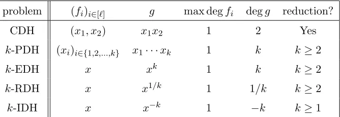
Table 1: Applicability of our technique in cyclic groups

problem (fi)i∈[ℓ] g max degfi degg reduction?

CDH (x1, x2) x1x2 1 2 Yes

k-PDH (xi)i∈{1,2,...,k} x1· · ·xk 1 k k≥2

k-EDH x xk _{1 k k≥2}

k-RDH x x1/k 1 1/k k≥2

k-IDH x x−k 1 −k k≥1

Observe that the left hand side is a degree 2 monic polynomial; hence, a non-zero polynomial. Since the reduction algorithm Rgen knows a value of r, it is able to find all solutions forx in polynomial

time. By checking [x] =X, the reduction algorithmRgensuccessfully finds a correct solution of the

DL_G.

By combining with Lemmas1,2, and Theorem1, we are able to obtain an information theoretic lower bound for the CDH.

Theorem 2 (Generic Hardness of CDH). The computational Diffie-Hellman problem in

Defini-tion 2 is (t2/p, t)-hard in the generic group model.

4.2 Master Theorem in Cyclic Groups

In this subsection, we provide the following master theorem in cyclic groups to indicate the power of our technique.

Theorem 3 (Master Theorem in Cyclic Groups). DL_G ⇒alg GDH_G holds when the following conditions hold:

(1) deg_x1,...,xmfi(x1, . . . , xm, y1, . . . , yn)∈ {0,1} for alli∈ {1,2, . . . , ℓ},

(2) degg(x1, . . . , xm)∈ {/ 0,1}.

Before providing a proof, we summarize the CDH variants which we summarized in Section2.1

and the conditions of Theorem 3 in Table 1. As the table shows, CDH, k-PDH, k-EDH, k-RDH, and k-IDH simultaneously satisfy the conditions (1) and (2) in Theorem 3 (although there are restrictions of k). Hence, as immediate corollary of the master theorem, we are able to provide generic and tight reductions from the DL to thek-PDH, k-EDH,k-RDH, andk-IDH.

Then, we show a proof of Theorem 3. In advance, we claim that the condition (1) will be used to ensure that the reduction algorithm is able to produce all group elements of the GDH during a reduction, while both the conditions (1) and (2) will be used to ensure that the modular equation never becomes a zero polynomial.

Proof. We construct a generic and tight reduction algorithmRgen. Specifically, the reduction algo-rithm Rgen uses an algebraic adversary Aalg on the GDHG only once and constructs an algebraic

adversaryBalg :=R Aalg

The reduction algorithmRgenis given a group descriptionG:= (G, G, p) and an instance of the

DL_G, i.e., X:= [x]∈Gfor an unknown x∈Zp. Thanks to the condition (1), we use the notation

fi(x1, . . . , xm, y1, . . . , yn) =fiL(y1, . . . , yn)xˆ_i+fiR(y1, . . . , yn)

with some ˆi∈ {1,2, . . . , m} for all i∈ {1,2, . . . , ℓ}. Then, the reduction algorithmRgen creates an

instance of the GDH_G as follows: Pick random (r2, . . . , rm, s1, . . . , sn)

$

←Zm+n−1

p and compute

Xi =fiL(s1, . . . , sn)·(X+rˆ_iG) +fiR(s1, . . . , sn)·G

= [f_iL(s1, . . . , sn)·x+fiL(s1, . . . , sn)·rˆ_i+fiR(s1, . . . , sn)]∈G

for all i∈ {1,2, . . . , ℓ} by implicitly setting

(x1, x2, . . . , xm, y1, . . . , yn) = (x, x+r2, . . . , x+rm, s1, . . . , sn).

Here, we use the notation r1 = 0 for simplicity. Then, the reduction algorithm Rgen gives a

group description G := (G, G, p) and group elements (X1, . . . , Xℓ) ∈ Gℓ to Aalg. Observe that

(X1, . . . , Xℓ) is a valid GDH instance since (x2, . . . , xm) is independently distributed ofx1to uniform inZm_p−1 from Aalg’s view. Hence, an algebraic adversary Aalg outputs a correct solution [Z]⃗z with an advantageAdvGDH_G,Aalg and a running time TimeGDH_G,Aalg.

Next, the reduction algorithm Rgen uses [Z]⃗z output by an algebraic adversary Aalg on the GDH_G and computes a solution of theDL_G. Assume the output is a correct solution of the GDH, i.e., Z = [g(x1, . . . , xm)]. It holds with probability AdvGDH_G,Aalg. Then, the representation vector

⃗

z:= (z0, z1, . . . , zℓ) satisfies

[g(x1, . . . , xm)]

=z0G+z1X1+· · ·+zℓXℓ

= [z0+

ℓ

∑

i=1

zifi(x1, . . . , xm, y1, . . . , yn)]

= [z0+ ℓ

∑

i=1 zi

(

f_iL(s1, . . . , sn)·x+fiL(s1, . . . , sn)·rˆi+f

R

i (s1, . . . , sn)

)

]

= [

( _ℓ ∑

i=1

zifiL(s1, . . . , sn)

)

x+z0+

ℓ

∑

i=1 zi

(

f_iL(s1, . . . , sn)·rˆ_i+fiR(s1, . . . , sn)

)

].

Hence, the reduction algorithm Rgen obtains the following univariate equation modulo a primep:

g(x, x+r2, . . . , x+rm)

=

( _ℓ ∑

i=1

zifiL(s1, . . . , sn)

)

x+z0+

ℓ

∑

i=1 zi

(

f_iL(s1, . . . , sn)·rˆ_i+fiR(s1, . . . , sn)

)

modp.

By combining with Lemmas1,2, and Theorem3, we are able to obtain an information theoretic lower bound for the GDH as follows.

Theorem 4(Generic Hardness of GDH). The generalized Diffie-Hellman problem in Definition7is

(t2/p, t)-hard in the generic group model if the conditions (1) and (2) of Theorem3 simultaneously

hold.

5

Reductions for Diffie-Hellman Variants in Symmetric Bilinear

Groups

In this section, we show generic and tight reductions from the bilinear discrete logarithm (BDL) problem to the computational bilinear Diffie-Hellman (CBDH) problem and its variants in an algebraic bilinear group model which we define in Section5.1. In Section5.2, we provide a reduction from the BDL to the CBDH. Finally, we provide our master theorem in Section5.3.

5.1 Algebraic Symmetric Bilinear Group Model

In advance of the reduction, we define an algebraic symmetric bilinear algorithm. The definition is analogous to Definition 29 in the sense that the algebraic symmetric bilinear algorithm is able to output only group elements which are derived from group additions inG, group multiplications in GT, and pairing e of given elements. Furthermore, the algebraic symmetric bilinear algorithm should also output arepresentation which indicates how output group elements are calculated. In this paper, we study computational problems in bilinear groups whose solutions Z are elements in

GT. Hence, we define a representation so that it records howZ is computed by group multiplications of given elements in GT and pairing of given elements in G. We formally provide a definition as follows.

Definition 30 (Algebraic Symmetric Bilinear Algorithm). An algorithm Aalg executed in an

alge-braic security gameG_G for G:= (G,GT, G, e, p) is calledalgebraicif for all group elementsZ ∈GT that Aalg outputs, it additionally return the representation of Z with respect to given group ele-ments. Specifically, if X⃗ := (X0, . . . , Xk) ∈ Gk+1, where X0 := G, and Y⃗ := (Y1, . . . , Yℓ) ∈ GℓT are the list of group elements that Aalg has received so far, then Aalg must also return a vector

⃗

z:= ((zi,j)0≤i≤j≤k,(zi′)1≤i≤ℓ)∈Z

(k+1)(k+2)

2 +ℓ

p such thatZ =

(∏

0≤i≤j≤ke(Xi, Xj)zi,j

) ·(∏ℓ

i=1Y

z′_i i

)

. We denote such an output as [Z]⃗z.

We note that the CBDH, k-PBDH, k-EBDH,k-RBDH, and k-IBDH do not take elements in

GT as the input. Therefore, the algorithm outputs Z along with a vector⃗z∈Z

(k+1)(k+2) 2

p .

5.2 BDL to CBDH Reduction via Affine Embedding

In this subsection, we extend the approach in Section 4 and prove the following reduction via the affine embedding.

Theorem 5. BDL_G ⇒alg BDH_G.

Proof. We construct a generic and tight reduction algorithm Rgen. Specifically, the reduction

al-gorithm Rgen uses an algebraic adversary Aalg on the BDH_G only once and construct an algebraic adversaryBalg :=R

Aalg

The reduction algorithm Rgen is given a bilinear group descriptionG := (G,GT, G, e, p) and an instance of the BDL_G, i.e., X := [x]∈G for an unknown x∈Zp. Then, the reduction algorithm

Rgencreates an instance of the BDHG as follows: Pick a random (r, s)

$

←Z2

p and compute

(X2=X+rG= [x+r], X3 =X+sG= [x+s])∈G2,

then set

(X1 =X, X2, X3)∈G3.

The reduction algorithm Rgen gives a bilinear group description G := (G,GT, G, e, p) and group elements (X1, X2, X3) ∈ G3 to Aalg. Observe that (X1, X2, X3) is a valid CBDH instance since

(x2, x3) is independently distributed of x to uniform in Z2_p from Aalg’s view. Hence, an algebraic

adversary Aalg outputs a correct solution [Z]⃗z with an advantage AdvBDH_G,Aalg and a running time TimeBDH_G,A

alg.

Next, the reduction algorithm Rgen uses [Z]⃗z output by an algebraic adversary Aalg on the

BDH_G and computes a solution of the BDL_G. Assume the output is a correct solution of the CBDH, i.e., Z = e(G, G)x1x2x3_{. It holds with probability Adv}BDH

G,Aalg. Then, we use X0 := [1] for

notational convenience and the representation vector ⃗z:= (zi,j)0≤i≤j≤3 satisfies

[x1x2x3]T = [x(x+r)(x+s)]T

= ∏

0≤i≤j≤3

e(Xi, Xj)zi,j

= [z0,0+z0,1x+z0,2(x+r) +z0,3(x+s) +z1,1x2+z1,2x(x+r) +z1,3x(x+s)

+z2,2(x+r)2+z2,3(x+r)(x+s) +z3,3(x+s)2]T.

Hence, the reduction algorithm Rgen obtains the following univariate equation modulo a primep:

x(x+r)(x+s)

=z0,0+z0,1x+z0,2(x+r) +z0,3(x+s) +z1,1x2+z1,2x(x+r)

+z1,3x(x+s) +z2,2(x+r)2+z2,3(x+r)(x+s) +z3,3(x+s)2 mod p

⇔ x3+ (r+s−z1,1−z1,2−z1,3−z2,2−z2,3−z3,3)x2

+ (rs−z0,1−z0,2−z0,3−rz1,2−sz1,3−2rz2,2−(r+s)z2,3−2sz3,3)x

−z0,0−rz0,2−sz0,3−r2z2,2−rsz2,3−s2z3,3 = 0 mod p.

Observe that the left hand side is a degree 3 monic polynomial; hence, a non-zero polynomial. Since the reduction algorithm Rgen knows values ofr and s, it is able to find all solutions forx in polynomial time. By checking [x] = X, the reduction algorithm Rgen successfully finds a correct

solution of the BDL_G.

By combining with Lemmas1,2, and Theorem5, we are able to obtain an information theoretic lower bound for the CBDH.

Table 2: Applicability of our technique in symmetric bilinear groups

problem (fi)i∈{1,2,...,k} h max degfi degh reduction?

CBDH (xi)i∈[3] x1x2x3 1 3 Yes

k-PBDH (xi)i∈{1,2,...,k} x1· · ·xk 1 k k≥3

k-EBDH x xk _{1 k k≥3}

k-RBDH x x1/k 1 1/k k≥2

k-IBDH x x−k 1 −k k≥1

5.3 Master Theorem in Symmetric Bilinear Groups

In this subsection, we provide the following master theorem in bilinear groups to indicate the power of our technique.

Theorem 7(Master Theorem in Bilinear Groups). BDL_G⇒alg GBDH_G holds when the following conditions hold:

(1) deg_x1,...,xmfi(x1, . . . , xm, y1, . . . , yn)∈ {0,1} for alli∈ {1,2, . . . , k},

(2) deg_x1,...,xmgi(x1, . . . , xm, y1, . . . , yn)∈ {0,1,2} for all i∈ {1,2, . . . , ℓ},

(3) degh(x1, . . . , xm)∈ {/ 0,1,2}.

Before providing a proof, we summarize the CBDH variants which we summarized in Section2.2

and the conditions of Theorem7 in Table 2. Since these problems do not take group elements in

GT as the input, we omit the condition (2) in the table. As the table shows, CBDH, k-PBDH,

k-EBDH, k-RBDH, and k-IBDH simultaneously satisfy the conditions (1) and (3) in Theorem 7

(although there are restrictions ofk). Hence, as immediate corollary of the master theorem, we are able to provide generic and tight reductions from the BDL to the k-PBDH, k-EBDH, k-RBDH, and k-IBDH.

Then, we show a proof of Theorem 7. In advance, we claim that the conditions (1) and (2) will be used to ensure that the reduction algorithm is able to produce all group elements of the GBDH during a reduction, while all the conditions (1), (2), and (3) will be used to ensure that the modular equation never becomes a zero polynomial.

Proof. We construct a generic and tight reduction algorithmRgen. Specifically, the reduction algo-rithmRgenuses an algebraic adversary Aalg on theGBDHG only once and constructs an algebraic

adversaryBalg :=RAgenalg on the BDLG.

The reduction algorithm Rgen is given a bilinear group descriptionG := (G,GT, G, e, p) and an instance of theBDL_G, i.e.,X := [x]∈Gfor an unknown x∈Zp. Thanks to the condition (1), we use the notation

fi(x1, . . . , xm, y1, . . . , yn) =fiL(y1, . . . , yn)xˆi+f

R

i (y1, . . . , yn)

with some ˆi ∈ {1,2, . . . , m} for all i ∈ {1,2, . . . , k}. Thanks to the condition (2), we use the notation

with some ˆi1,ˆi2,ˆi3 ∈ {1,2, . . . , m} for all i ∈ {1,2, . . . , ℓ}. Then, the reduction algorithm Rgen

creates an instance of theGBDH_G as follows: Pick random (r2, . . . , rm, s1, . . . , sn)

$

←Zm+n−1

p and

compute

Xi =fiL(s1, . . . , sn)·(X+rˆ_iG) +fiR(s1, . . . , sn)·G

= [f_iL(s1, . . . , sn)·(x+rˆ_i) +fiR(s1, . . . , sn)]∈G for all i∈ {1,2, . . . , k}and

Yi =e(X+rˆ_i1G, X+rˆ_i2G)g

L

i(s1,...,sn)·_{e(G, X+rˆ} i3G)

gM

i(s1,...,sn)·_{e(G, G)}giR(s1,...,sn)

= [g_iL(s1, . . . , sn)·(x+rˆi1)(x+rˆi2) +g

M

i (s1, . . . , sn)·(x+rˆi3) +g

R

i(s1, . . . , sn)]T ∈GT for all i∈ {1,2, . . . , ℓ} by implicitly setting

(x1, x2, . . . , xm, y1, . . . , yn) = (x, x+r2, . . . , x+rm, s1, . . . , sn).

Here, we use the notation r1 = 0 for simplicity. Then, the reduction algorithm Rgen gives a bilinear group descriptionG:= (G,GT, G, e, p) and group elements (X1, . . . , Xk, Y1, . . . , Yℓ)∈Gk×

Gℓ

T to Aalg. Observe that (X1, . . . , Xk, Y1, . . . , Yℓ) is a valid GBDH instance since (x2, . . . , xm) is independently distributed ofx1to uniform inZm_p −1 fromAalg’s view. Hence, an algebraic adversary

Aalg outputs a correct solution [Z]⃗z with an advantageAdvGBDH_G,Aalg and a running time Time

GBDH

G,Aalg .

Next, the reduction algorithm Rgen uses [Z]⃗z output by an algebraic adversary Aalg on the

GBDH_G and computes a solution of the BDL_G. Assume the output is a correct solution of the GBDH, i.e., Z = [h(x1, . . . , xm)]T. It holds with probabilityAdvGBDH_G,Aalg . Then, the representation

vector⃗z:= ((zi,j)0≤i≤j≤k,(zi′)1≤i≤ℓ) satisfies

[h(x1, . . . , xm)]T

=



 ∏

0≤i≤j≤k

e(Xi, Xj)zi,j

 _·



 ∏

1≤i≤ℓ

Yzi′ i

 

= [ ∑

0≤i≤j≤k

zi,jfi(x1, . . . , xm, y1, . . . , yn)·fj(x1, . . . , xm, y1, . . . , yn) + ℓ

∑

i=1

z_i′gi(x1, . . . , xm, y1, . . . , yn)]T

= [ ∑

0≤i≤j≤k

zi,j

(

f_iL(s1, . . . , sn)·(x+rˆ_i) +fiR(s1, . . . , sn)

) (

f_jL(s1, . . . , sn)·(x+rˆ_j) +fjR(s1, . . . , sn)

)

+ ℓ

∑

i=1 z_i′

(

gL_i(s1, . . . , sn)·(x+rˆ_i1)(x+rˆ_i2) +gMi (s1, . . . , sn)·(x+rˆ_i3) +gRi(s1, . . . , sn)

)

]T

= [



 ∑

0≤i≤j≤k

zi,jfiL(s1, . . . , sn)fjL(s1, . . . , sn) + ℓ

∑

i=1

z′_igL_i(s1, . . . , sn)

 x2

+



 ∑

0≤i≤j≤k

zi,j

(

f_iL(s1, . . . , sn)(fjL(s1, . . . , sn)·rˆ_j+fjR(s1, . . . , sn))

+f_jL(s1, . . . , sn)(fiL(s1, . . . , sn)·rˆ_i+fiR(s1, . . . , sn))

)

+ ℓ

∑

i=1 z_i′

(

g_iL(s1, . . . , sn)·(rˆ_i1 +rˆ_i2) +giM(s1, . . . , sn)

))