Synthesizing a Broad Beam for an
Atmospheric Radar
K.Lakshmi Anitha1, Dr.N.Deepika Rani2, Prof.G.T.Rao3
PG Student, Dept. of ECE, GVP College of Engineering (A), Visakhapatnam, Andhra Pradesh, India1
Associate Professor, Dept. of ECE, GVP College of Engineering (A), Visakhapatnam, Andhra Pradesh, India2
Professor, Dept. of ECE, GVP College of Engineering (A), Visakhapatnam, Andhra Pradesh, India3
ABSTRACT:Atmospheric radars use phased array for monitoring the phenomenon at different layers by sounding the
layers and processing the information from echoes. Certain atmospheric conditions require this monitoring to be done over a wide spectrum and also in a wider range of coverage. To sound wider areas, radars need to adapt to beam broadening techniques, so that echo processing can be done for better SNR. Broad beam pattern is achieved using phase only synthesis in principal planes. This paper describes the phase only pattern synthesis for the active phased array antenna using Differential Evolution (DE) algorithm. The atmospheric radar should have broad beam to get data from large area in turbulent conditions. Broadening of 32 X 32 planar array can be demonstrated using Differential Evolution (DE) algorithm.
KEYWORDS: Phase only pattern synthesis, Genetic Algorithm, Differential Evolution, Active phased array antenna.
I.INTRODUCTION
Broad beam is used in Atmospheric radars. Broad beam is used to obtain data from large area in turbulent conditions. It is obtained using phase only pattern synthesis for the active phased array antenna using genetic algorithm [1]. Phase excitations for beam broadening are obtained using Differential Evolution algorithm [2]. Symmetric distribution of phases are considered [3].
II.PLANAR ARRAY
Consider M X N element planar array of isotropic radiators as shown in Fig. 1.
Fig.1. Geometry of M X N element planar array [7]
( ) = ( )( ∅) ( )( ∅)
where is excitation of ( , ) element, dx and dy are inter element spacing in x and y directions respectively, M
and N are number of elements along x and y directions , k = , θ is angle from z-axis and is angle from x-axis.
The excitation can be expressed as
= ∗
If amplitude excitation of the entire array is uniform then
= exp( ∗ )
= ( ∗ )
=
∗( ) ∗( )
∗( ) ∗( )
⋯ ∗( )
⋯ ∗( )
⋮ ⋮
∗( ) ∗( )
⋮ ⋮ ⋯ ∗( )
In a symmetric M X M planar array phase excitations and are equal and only M/2 phases in are enough
to achieve phase excitations of all elements in planar array.
The optimum values of phase excitations are computed using DE to achieve beam broadening. The objective
function ( ), used for beam broadening, can be expressed as :
( ) = 0.22 1 −−905 ≤≤ ≤≤ −55 0.22 5 ≤ ≤90
Cost function ∆, which is defined as difference in the specified and achieved antenna pattern side lobe levels summed
across θ, can be expressed as:
1
2
N
y
1
2
M
x
d
x∆ = ( )− ( ) + | ( )− ( )| + ( )− ( )
Outside the main beam region, if (AF( )− ( )) is negative at a particular value, then (AF( )− ( )) will be
considered to be zero for calculation of cost function. Here , and are weighting factors of cost function. The
weighting factors are represented by
= 1
AF(θ) is radiation pattern for the given phase excitations.
III.DIFFERENTIAL EVOLUTION
Differential evolution is a Stochastic, population-based optimization algorithm introduced by Storn and Price. DE optimizes a problem by maintaining a population of solutions and generating new solutions by combining existing ones according to the Cost function, and then keeping the resulting solution as the best one. The DE is explained in the following steps.
Initialization:
The generation number is set to t=0 and a population of Ps individuals is randomly initialized in D-dimensional search
space as Pt ={X1(t);X2(t);... ..Xps(t)} where ( )is target vector and is given by
Xi(t)=[xi,1(t),xi,2(t),xi,3(t),...,xi,D(t)] and each individuals are uniformly distributed in the domain [Xmin,Xmax].
Cost Function Evaluation
A cost function rating the performance is evaluated for each member of the population.
Differential Mutation
After fitness function evaluation, DE creates a mutant vector for each individual Vi(t)=[vi,1(t),vi,2(t),....vi,D(t)]
DE creates a mutant vector by adding the weighted difference between two population vectors to a third vector. This operation is called mutation. The requirement of creating mutant vector decides the efficient algorithms for best crossover solution.
= + . ( − ) ≠ 1≠ 2
where ( ) is mutant vector. , are random but mutually different donor vectors in the population. is the
individual vector that has the best fitness value in the current population and Mutation factor F [0, 2] controls the
amplification of the differential variation ( − ) target vector.
Crossover
To enhance the potential diversity of the population, a crossover operation is done using mutant vector exchanging its
components with the target vector to form the trial vector ( ) under “binomial” crossover operati.on to form the trial
vector ( )= , ( ), , ( ), … … , ( )
, = ,
(0,1)≤ ( = )
, ℎ
Where j=1,2,...D, CR is cross over rate in range [0,1] ‘jrand ’ is a randomly chosen index to ensure that the trial vector
is not a duplicate of .
Selection
Selection operation determines which one of the target and the trial vector survives to the next generation i.e. at
( )= ( )
, ( ) ≤ ( )
( ), ℎ
Hence the population either gets better or remains constant, but never deteriorates. Compute ( ) among
individuals at current generation as follows:
( )= { ,…, } ( )
For various generations, ( ) is repeated and the final ( ) is computed after the terminal criteria is met.
The terminal criterion is of two kinds. One is convergence criterion that the variation in the minimum or maximum between two previous generations should be less than some specified. The other is an upper bound on the number of generations. There can be a hybrid version of these two criteria.
Beam broadening in both planes is explained from a planar array with 32 X 32 elements. The inter element spacing along
both x and y is 0.7 λ.
IV.RESULT AND DISCUSSION
Consider a broadside uniform planar array of 32 X 32 elements with inter element spacing of 0.7λ in both x and y
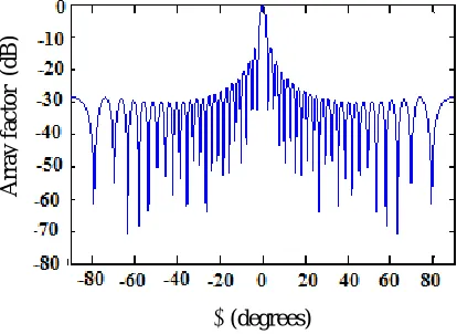
directions. Radiation pattern of the uniform planar array of 32 X 32 elements with θ varying from -900 to 900 and ϕ =00
is shown in Fig.2.
Fig 2: Radiation pattern of 32 X 32 broadside uniform planar array with 0.7λ spacing
From Fig.2 it is observed that -3dB beamwidth is 2.5 and peak side lobe level is -13.4dB.
To achieve beam broadening, optimum phase excitations are computed using DE. For 32 X 32 planar array only
M/2=16 phases are considered as the individuals in DE population. These phases are mirrored symmetrically to get 32
phase excitations. The limits phase excitation are considered as 00 and 3600.
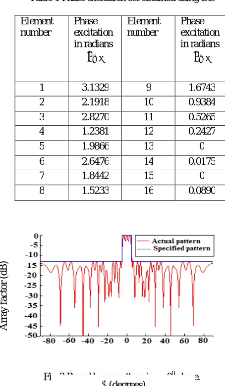
The parameters of the differential evolution are taken as follows: Mutation factor F=0.8, Crossover constant CR=0.98, Population size Ps=100, Weighting factors 0.8, 0.1 and 0.1 respectively. Table 1 shows optimum M/2 phase excitations
obtained using DE. Fig. 3 and Fig. 4 show desired broad beam pattern and pattern obtained using DE in =00 plane and
900 plane respectively.
(degrees)
A
rra
y
fa
c
tor
Table 1 Phase excitation set obtained using DE
Element number
Phase excitation in radians
Element number
Phase excitation in radians
1 3.1329 9 1.6743
2 2.1918 10 0.9384
3 2.8270 11 0.5265
4 1.2381 12 0.2427
5 1.9866 13 0
6 2.6476 14 0.0175
7 1.8442 15 0
8 1.5233 16 0.0890
Fig 3 Broad beam pattern in =00 plane.
Fig 3 shows broad beam pattern in =00 plane. The obtained beamwidth of broad beam is 10
Fig 4 Broad beam pattern in =900 plane
(degrees)
A
rra
y
fa
c
tor
(dB
)
(degrees)
A
rra
y
fa
c
tor
(dB
Fig 3 shows broad beam pattern in =00 plane. The obtained beamwidth of broad beam is 10
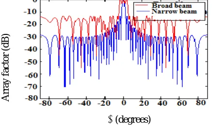
Fig. 5 Comparison of narrow beam and broad beam in =00 plane.
From fig 5 it is observed that beam is broadened from 2.5 to 10
Fig. 6 Comparison of narrow beam and broad beam in =900 plane.
From Figures 5 and 6, it is observed that the -3dB beamwidth of broad beam is 100 and first side lobe level is -13.2dB.
The beam is broadened four times when compared to narrow beam pattern.
Fig 7 Convergence curve for Cost function
(degrees)
A
rra
y
fa
c
tor
(dB
)
(degrees)
A
rra
y
fa
c
tor
(dB
)
Iteration
C
os
t
fu
nc
ti
Figure 7 shows the convergence curve for cost function. It can be observed from Fig. 7 that DE takes 31 iterations for getting the best fit value.
.
V. CONCLUSION
In this paper, the global search ability of DE is used to achieve beam broadening with the approach of phase-only by constructing an initial phase of linear distribution for a uniform planar array antenna. Here beam broadening by a factor of four in both the planes has been illustrated, which will also provide better beam efficiency. Beam broadening
capability is demonstrated from 2.50 to 100. In this method 32 symmetric phases are synthesized for DE application.
The simulated pattern of a planar array is found to be in close agreement with the desired beam shape.
REFERENCES
[1] Pramod kumar, A.K Singh, Phase only pattern synthesis for antenna array using genetic algorithm for radar application, Indian Journal of Radio and space physics, Vol 42, August 2013
[2] Rainer Storn, Kenneth Price, Differential Evolution, A simple and efficient heuristic for global optimization over continuous spaces, Journal of
Global optimization,1997.
[3] K.H. Sayidmarie, and Q.H. Sultan,”Synthesis of wide beam array pattern using random phase weights”, International Journal of
Electromagnetics and Applications, vol.3, No 6, 2013.
[4] Kerce J C, Brown G C & Mitchell M A, Extremes beam broadening using phase only synthesis, Fourth IEEE workshop on Sensor Array and
Multi-channel processing, Waltham, MA (USA), 12-14 July 2006
[5] Khzmalyan A D, Phase only control of an array pattern: Beam shaping and monopulse nulling , IEEE International Symposium on Phased
Array Systems and Technology (IEEE, New York), 2003, pp 577-582.
[6] Haupt R L, An introduction to genetic algorithms for electromagnetic, IEEE Antennas Propag Mag (USA), 37 (1995) pp 7–15.