New Complexity Trade-Offs for the (Multiple)
Number Field Sieve Algorithm in Non-Prime
Fields
Palash Sarkar and Shashank Singh
Applied Statistics Unit Indian Statistical Institute
[email protected], [email protected]
Abstract. The selection of polynomials to represent number fields cru-cially determines the efficiency of the Number Field Sieve (NFS) algo-rithm for solving the discrete logaalgo-rithm in a finite field. An important re-cent work due to Barbulescu et al. builds upon existing works to propose two new methods for polynomial selection when the target field is a non-prime field. These methods are called the generalised Joux-Lercier (GJL) and the Conjugation methods. In this work, we propose a new method (which we denote asA) for polynomial selection for the NFS algorithm in fieldsFQ, withQ=pn and n >1. The new method both subsumes
and generalises the GJL and the Conjugation methods and provides new trade-offs for bothncomposite andnprime. Let us denote the variant of the (multiple) NFS algorithm using the polynomial selection method “X” by (M)X. Asymptotic analysis is performed for both the
NFS-Aand the MNFS-Aalgorithms. In particular, whenp=LQ(2/3, cp), for
cp∈[3.39,20.91], the complexity of NFS-Ais better than the complexi-ties of all previous algorithms whether classical or MNFS. The MNFS-A
algorithm provides lower complexity compared to NFS-Aalgorithm; for
cp ∈ (0,1.12]∪[1.45,3.15], the complexity of MNFS-A is the same as that of the MNFS-Conjugation and forcp ∈/ (0,1.12]∪[1.45,3.15], the complexity of MNFS-Ais lower than that of all previous methods.
1
Introduction
Let G =hgi be a finite cyclic group. The discrete log problem (DLP) in G is the following. Given (g,h), compute the minimum non-negative integer e such that h= ge. For appropriately chosen groups G, the DLP in G is believed to be computationally hard. This forms the basis of security of many important cryptographic protocols.
For small characteristic fields, the FFS algorithm leads to a quasi-polynomial running time [6]. Using the FFS algorithm outlined in [15, 6], Granger et al. [12] reported a record computation of discrete log in the binary extension fieldF29234.
FFS also applies to the medium characteristic fields. Some relevant works along this line are reported in [18, 14, 25].
For medium to large characteristic finite fields, the NFS algorithm is the state-of-the-art. In the context of the DLP, the NFS was first proposed by Gor-don [11] for prime order fields. The algorithm proceeded via number fields and one of the main difficulties in applying the NFS was in the handling of units in the corresponding ring of algebraic integers. Schirokauer [26, 28] proposed a method to bypass the problems caused by units. Further, Schirokauer [27] showed the application of the NFS algorithm to composite order fields. Joux and Lercier [17] presented important improvements to the NFS algorithm as applicable to prime order fields.
Joux, Lercier, Smart and Vercauteren [19] later showed that the NFS algo-rithm is applicable to all finite fields. Since then, several works [20, 5, 13, 24] have gradually improved the NFS in the context of medium to large characteristic fi-nite fields.
The efficiency of the NFS algorithm is crucially dependent on the properties of the polynomials used to construct the number fields. Consequently, poly-nomial selection is an important step in the NFS algorithm and is an active area of research. The recent work [5] by Barbulescu et al. extends a previous method [17] for polynomial selection and also presents a new method. The ex-tension of [17] is called the generalised Joux-Lercier (GJL) method while the new method proposed in [5] is called the Conjugation method. The paper also provides a comprehensive comparison of the trade-offs in the complexity of the NFS algorithm offered by the various polynomial selection methods.
The NFS based algorithm has been extended to multiple number field sieve algorithm (MNFS). The work [8] showed the application of the MNFS to medium to high characteristic finite fields. Pierrot [24] proposed MNFS variants of the GJL and the Conjugation methods. For more recent works on NFS we refer to [7, 22, 4].
Our contributions: In this work, we build on the works of [17, 5] to propose a new method of polynomial selection for NFS overFpn. The new method both
subsumes and generalises the GJL and the Conjugation methods. There are two parameters to the method, namely a divisor dof the extension degreen and a parameterr≥kwherek=n/d.
Ford= 1, the new method becomes the same as the GJL method. Ford=n
andr=k= 1, the new method becomes the same as the Conjugation method. Ford=nand r >1; or, for 1< d < n, the new method provides polynomials which leads to different trade-offs than what was previously known. Note that the case 1< d < ncan arise only whennis composite, though the cased=nand
Following the works of [5, 24] we carry out an asymptotic analysis of new method for the classical NFS as well as for MNFS. For the medium and the large characteristic cases, the results for the new method are exactly the same as those obtained for existing methods in [5, 24]. For the boundary case, however, we obtain some interesting asymptotic results. LettingQ=pn, the subexponential expressionLQ(a, c) is defined to be the following:
LQ(a, c) = exp (c+o(1))(lnQ)a(ln lnQ)1−a. (1) Write p = LQ(2/3, cp) and let θ0 and θ1 be such that the complexity of the MNFS-Conjugation method isLQ(1/3, θ0) and the complexity of the MNFS-GJL method isLQ(1/3, θ1). As shown in [24],LQ(1/3, θ0) is the minimum complexity of MNFS†while forcp>4.1, complexity of new method (MNFS-A) is lower than the complexityLQ(1/3, θ1) of MNFS-GJL method.
The classical variant of the new method, (i.e., NFS-A) itself is powerful enough to provide better complexity than all previously known methods, whether classical or MNFS, forcp∈[3.39,20.91]. The MNFS variant of the new method provides lower complexity compared to the classical variant of the new method for allcp.
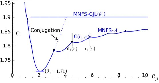
The complexity of MNFS-Awithk= 1 and using linear sieving polynomials can be written as LQ(1/3,C(cp, r)), where C(cp, r) is a function of cp and a parameterr. For every integerr≥1, there is an interval [0(r), 1(r)] such that for cp ∈ [0(r), 1(r)], C(cp, r) < C(cp, r0) for r 6= r0. Further, for a fixed r,
Fig. 1.Complexity plot for MNFS boundary case
let C(r) be the minimum value of C(cp, r) over all cp. We show that C(r) is monotone increasing forr≥1;C(1) =θ0; and thatC(r) is bounded above by
θ1 which is its limit asrgoes to infinity. So, for the new method the minimum †
complexity is the same as MNFS-Conjugation method. On the other hand, asr
increases, the complexity of MNFS-Aremains lower than the complexities of all the prior known methods. In particular, the complexity of MNFS-Ainterpolates nicely between the complexity of the MNFS-GJL and the minimum possible complexity of the MNFS-Conjugation method. This is depicted in Figure 1. In Figure 4 of Section 8.1, we provide a more detailed plot of the complexity of MNFS-Ain the boundary case.
The complete statement regarding the complexity of MNFS-Ain the bound-ary case is the following. Forcp∈(0,1.12]∪[1.45,3.15], the complexity of MNFS-Ais the same as that of MNFS-Conjugation; forcp∈/(0,1.12]∪[1.45,3.15], the complexity of MNFS-Ais lower than that of all previous methods. In particular, the improvements forcpin the range (1.12,1.45) is obtained usingk= 2 and 3; while the improvements for cp >3.15 is obtained using k= 1 and r >1. In all cases, the minimum complexity is obtained using linear sieving polynomials.
2
Background on NFS for Non-Prime Fields
We provide a brief sketch of the background on the variant of the NFS algorithm that is applicable to the extension fields FQ, where Q = pn, p is a prime and
n >1. More detailed discussions can be found in [17, 5].
Following the structure of index calculus algorithms, NFS has three main phases, namely, relation collection (sieving), linear algebra and descent. Prior to these, is the set-up phase. In the set-up phase, two number fields are constructed and the sieving parameters are determined. The two number fields are set up by choosing two irreducible polynomialsf(x) and g(x) over the integers such that their reductions modulo p have a common irreducible factor ϕ(x) of degree n
over Fp. The field Fpn will be considered to be represented by ϕ(x). Let g be
a generator ofG=F?pn and let qbe the largest prime dividing the order of G.
We are interested in the discrete log of elements ofGto the basegmodulo this largest primeq.
The choices of the two polynomialsf(x) andg(x) are crucial to the algorithm. These greatly affect the overall run time of the algorithm. Let α, β ∈ C and
m∈Fpn be the roots of the polynomialsf(x), g(x) and ϕ(x) respectively. We
further letl(f) andl(g) denote the leading coefficient of the polynomials f(x) and g(x) respectively. The two number fields and the finite field are given as follows.
K1=Q(α) = Q[x]
hf(x)i,K2=Q(β) =
Q[x]
hg(x)i andFpn=Fp(m) =
Fp[x]
hϕ(x)i.
of algebraic integersOi. These integer rings provide a nice way of constructing a factor basis and moreover, unique factorisation of ideals holds over these rings.
The factor basisF=F1∪ F2is chosen as follows.
F1=
prime idealsq1,j in O1, either having norm less thanB or lying above the prime factors of l(f)
F2=
prime idealsq2,j inO2, either having norm less thanB or lying above the prime factors ofl(g)
whereBis the smoothness bound and is to be chosen appropriately. An algebraic integer is said to be B-smooth if the principal ideal generated by it factors into the prime ideals of norms less than B. As mentioned in the paper [5], independently of choice of f and g, the size of the factor basis is B1+o(1). For asymptotic computations, this is simply taken to be B. The work flow of NFS can be understood by the diagram in Figure 2.
Z[x]
Z(α) Z(β)
Fp(m) α
7→ x x7→ β
α7→ m
m 7→ β
Fig. 2.A work-flow of NFS.
A polynomialφ(x)∈Z[x] of degree at mostt−1 (i.e. havingtcoefficients) is chosen and the principal ideals generated by its images in the two number fields are checked for smoothness. If both of them are smooth, then
φ(α)O1=
Y
j
q1,jej and φ(β)O2=
Y
j
q2,je 0
j (2)
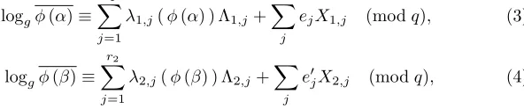
whereq1,j andq2,j are prime ideals inF1andF2respectively. Fori= 1,2, lethi denote the class number of Oi and ri denote the torsion-free rank ofOi?. Then, for someεi,j ∈qi,j and unitsui,j∈ Oi?, we have
loggφ(α)≡ r1
X
j=1
λ1,j(φ(α) ) Λ1,j+
X
j
ejX1,j (modq), (3)
loggφ(β)≡ r2
X
j=1
λ2,j(φ(β) ) Λ2,j+
X
j
e0jX2,j (modq), (4)
of prime idealqi,jandλi,j:Oi 7→Z/qZis Schirokauer map [26, 28, 19]. We skip
the details of virtual logarithms and Schirokauer maps, as these details will not affect the polynomial selection problem considered in this work.
Sinceφ(α) =φ(β), we have
Pr1
j=1λ1,j(φ(α) ) Λ1,j+PjejX1,j ≡P r2
j=1λ2,j(φ(β) ) Λ2,j+Pje0jX2,j(modq) (5)
The relation given by (5) is a linear equation moduloq in the unknown virtual logs. More than (#F1+ #F2+r1+r2) such relations are collected by sieving over suitableφ(x). The linear algebra step solves the resulting system of linear equations using either the Lanczos or the block Wiedemann algorithms to obtain the virtual logs of factor basis elements.
After the linear algebra phase is over, the descent phase is used to compute the discrete logs of the given elements of the field Fpn. For a given element y
of Fpn, one looks for an element of the form yigj, for somei, j ∈N, such that
the principal ideal generated by preimage of yigj in O1, factors into prime ideals of norms bounded by some boundB1 and of degree at mostt−1. Then the special-q descent technique [19] is used to write the ideal generated by the preimage as a product of prime ideals inF1, which is then converted into a linear equation involving virtual logs. Putting the value of virtual logs, obtained after linear algebra phase, the value of logg(y) is obtained. For more details and recent work on the descent phase, we refer to [19, 13].
3
Polynomial Selection and Sizes of Norms
It is evident from the description of NFS that the relation collection phase re-quires polynomialsφ(x)∈Z[x] whose images in the two number fields are simul-taneously smooth. For ensuring the smoothness of φ(α) and φ(β), it is enough to ensure that their norms viz, Res(f, φ) and Res(g, φ) areB-smooth. We refer to [5] for further explanations.
Using the Corollary 2 of Kalkbrener’s work [21], we have the following upper bound for the absolute value of the norm.
|Res(f, φ)| ≤κ(degf,degφ)kfkdegφ
∞ kφkdeg∞ f (6) where κ(a, b) = a+ba a+b−1
a
and kfk∞ is maximum of the absolute values of the coefficients of f.
Following [5], letE be such that the coefficients ofφare in−1 2E
2/t,1 2E
2/t
. So,kφk∞≈E2/tand the number of polynomialsφ(x) that is considered for the sieving isE2. Wheneverp=LQ(a, cp) witha > 13, we have the following bound on the Res(f, φ)×Res(g, φ) (for details we refer to [5]).
|Res(f, φ)×Res(g, φ)| ≈(kfk∞kgk∞)t−1E(degf+degg)2/t. (7)
The methods for choosingf andg result in the coefficients of one or both of these polynomials to depend onQ. So, the right hand side of (7) is determined byQandE. All polynomial selection algorithms try to minimize the RHS of (7). From the bound in (7), it is evident that during polynomial selection, the goal should be to try and keep the degrees and the coefficients of bothf andg to be small. Ensuring both degrees and coefficients to be small is a nontrivial task and leads to a trade-off. Previous methods for polynomial selections provide different trade-offs between the degrees and the coefficients. Estimates of Q-E trade-off values have been provided in [5] and is based on the CADO factoring software [3]. Table 1 reproduces these values whereQ(dd) represents the number of decimal digits inQ.
Table 1.Estimate ofQ-E values [5].
Q(dd) 100 120 140 160 180 200 220 240 260 280 300
Q(bits) 333 399 466 532 598 665 731 798 864 931 997
E(bits) 20.9 22.7 24.3 25.8 27.2 28.5 29.7 30.9 31.9 33.0 34.0
As mentioned in [5, 13], presently the following three polynomial selection methods provide competitive trade-offs.
1. JLSV1:Joux, Lercier, Smart, Vercauteren method [19]. 2. GJL:Generalised Joux Lercier method [23, 5].
3. Conjugation method[5].
Brief descriptions of these methods are given below.
JLSV1. Repeat the following steps untilf andgare obtained to be irreducible overZandϕis irreducible overFp.
1. Randomly choose polynomialsf0(x) andf1(x) having small coefficients with deg(f1)<deg(f0) =n.
2. Randomly choose an integer`to be slightly greater thand√pe. 3. Let (u, v) be the rational reconstruction of`inFp, i.e., `≡u/vmodp.
4. Define f(x) = f0(x) + `f1(x) and g(x) = vf0(x) +uf1(x) and ϕ(x) =
f(x) modp.
Note that deg(f) = deg(g) = n and both kfk∞ and kgk∞ are O p1/2 =
O Q1/(2n)and so (7) becomesE4n/tQ(t−1)/nwhich isE2nQ1/nfort= 2.
The heart of the GJL method is the following idea. Let ϕ(x) be a monic polynomial ϕ(x) = xn +ϕ
n−1xn−1+· · ·+ϕ1x+ϕ0 and r ≥ deg(ϕ) be an integer. Let n= deg(ϕ). Givenϕ(x) and r, define an (r+ 1)×(r+ 1) matrix
Mϕ,r in the following manner.
Mϕ,r=
p
. .. . ..
p ϕ0ϕ1· · ·ϕn−1 1
. .. . .. . ..
ϕ0 ϕ1 · · ·ϕn−11
(8)
The first n×n principal sub-matrix of Mϕ,r is diag[p, p, . . . , p] corresponding to the polynomials p, px, . . . , pxn−1. The lastr−n+ 1 rows correspond to the polynomialsϕ(x), xϕ(x), . . . , xr−nϕ(x).
Apply the LLL algorithm toMϕ,r and let the first row of the resulting LLL-reduced matrix be [g0, g1, . . . , gr−1, gr]. Define
g(x) =g0+g1x+· · ·+gr−1xr−1+grxr. (9) The notation
g= LLL (Mϕ,r) (10)
will be used to denote the polynomial g(x) given by (9). By construction,ϕ(x) is a factor ofg(x) modulo p.
The GJL procedure for polynomial selection is the following. Choose anr≥n
and repeat the following steps until f and g are irreducible over Z and ϕ is irreducible overFp.
1. Randomly choose a degree (r+ 1)-polynomialf(x) which is irreducible over
Zand having coefficients of sizeO(ln(p)) such thatf(x) has a factorϕ(x)
of degreenmodulopwhich is both monic and irreducible. 2. Letϕ(x) =xn+ϕ
n−1xn−1+· · ·+ϕ1x+ϕ0andMϕ,r be the (r+ 1)×(r+ 1) matrix given by (8).
3. Letg(x) = LLL (Mϕ,r).
The polynomial f(x) has degreer+ 1 and g(x) has degreer. The procedure is parameterised by the integer r.
The determinant ofM is pn and so from the properties of the LLL-reduced basis, the coefficients ofg(x) are of the orderO pn/(r+1)
=O Q1/(r+1)
. The coefficients off(x) areO(lnp).
Conjugation. Repeat the following steps untilf and g are irreducible overZ andϕis irreducible overFp.
1. Choose a quadratic monic polynomialµ(x), having coefficients of sizeO(lnp), which is irreducible overZand has a roottin Fp.
2. Choose two polynomials g0(x) and g1(x) with small coefficients such that degg1<degg0=n.
3. Let (u, v) be a rational reconstruction of tmodulop, i.e.,t≡u/vmodp. 4. Define g(x) =vg0(x) +ug1(x) andf(x) = Resy(µ(y), g0(x) +y g1(x)). Note that deg(f) = 2n, deg(g) =n, kfk∞ = O(lnp) and kgk∞ =O(p1/2) =
O(Q1/(2n)). In this case, the bound on the norm given by (7) isE6n/tQ(t−1)/(2n)
which becomesE3nQ1/(2n) fort= 2.
4
A Simple Observation
For the GJL method, while constructing the matrix M, the coefficients of the polynomial ϕ(x) are used. If, however, some of these coefficients are zero, then these may be ignored. The idea is given by the following result.
Proposition 1. Let n be an integer, d a divisor of n and k = n/d. Suppose
A(x)is a monic polynomial of degreek. Letr≥k be an integer and setψ(x) = LLL(MA,r). Define g(x) =ψ(xd)andϕ(x) =A(xd). Then
1. deg(ϕ) =n anddeg(g) =rd; 2. ϕ(x)is a factor ofg(x)modulo p; 3. kgk∞=pn/(d(r+1)).
Proof. The first point is straightforward. Note that by construction A(x) is a factor of ψ(x) modulop. So,A(xd) is a factor ofψ(xd) =g(x) modulo p. This shows the second point. The coefficients of g(x) are the coefficients of ψ(x). Following the GJL method, kψk∞ = pk/(r+1) = pn/(d(r+1)) and so the same
holds forkgk∞. This shows the third point. ut
Note that if we had defined g(x) = LLL(Mϕ,rd), then kgk∞ would have been
pn/(rd+1). Ford >1, the value ofkgk∞given by Proposition 1 is smaller.
A variant. The above idea shows how to avoid the zero coefficients of ϕ(x). A similar idea can be used to avoid the coefficients of ϕ(x) which are small. Suppose that the polynomialϕ(x) can be written in the following form.
ϕ(x) =ϕi1x
i1+· · ·+ϕ
ikx
ik+xn+ X
j /∈{i1,...,ik}
ϕjxj (11)
be zero. A (k+ 1)×(k+ 1) matrixM is constructed in the following manner.
M =
p
. .. . ..
p ϕi1ϕi2 · · ·ϕik1
(12)
The matrix M has only one row obtained from ϕ(x) and it is difficult to use more than one row. Apply the LLL algorithm to M and write the first row of the resulting LLL-reduced matrix as [gi1, . . . , gik, gn]. Define
g(x) = (gi1x
i1+· · ·+g
ikx
ik+g
nxn) +
X
j /∈{i1,...,ik,n}
ϕjxj. (13)
The degree ofg(x) isnand the bound on the coefficients ofg(x) is determined as follows. The determinant of M ispk and by the LLL-reduced property, each of the coefficients gi1, . . . , gik, gn isO(p
k/(k+1)) = O(Qk/(n(k+1))). Since ϕ j for
j /∈ {i1, . . . , ik} are allO(1), it follows from (13) that all the coefficients ofg(x) areO(Qk/(n(k+1))) and sokgk
∞=O(Qk/(n(k+1))).
5
A New Polynomial Selection Method
In the simple observation made in the earlier section, the non-zero terms of the polynomial g(x) are powers ofxd. This creates a restriction and does not turn out to be necessary to apply the main idea of the previous section. Once the polynomial ψ(x) is obtained using the LLL method, it is possible to substitute any degree dpolynomial with small coefficients forxand still the norm bound will hold. In fact, the idea can be expressed more generally in terms of resultants. AlgorithmAdescribes the new general method for polynomial selection.
The following result states the basic properties of AlgorithmA.
Proposition 2. The outputs f(x), g(x) and ϕ(x) of Algorithm A satisfy the following.
1. deg(f) =d(r+ 1);deg(g) =rdanddeg(ϕ) =n; 2. bothf(x)andg(x)haveϕ(x) as a factor modulop; 3. kfk∞=O(ln(p))andkgk∞=O(Q1/(d(r+1))).
Consequently,
|Res(f, φ)×Res(g, φ)| ≈(kfk∞kgk∞) t−1
×E2(degf+degg)/t
Algorithm:A: A new method of polynomial selection.
Input:p,n,d(a factor ofn) andr≥n/d.
Output:f(x),g(x) andϕ(x). Letk=n/d;
repeat
Randomly choose a monic irreducible polynomialA1(x) having the following properties: degA1(x) =r+ 1;A1(x) is irreducible over the integers;A1(x) has coefficients of sizeO(ln(p)); modulop,A1(x) has an irreducible factorA2(x) of degreek.
Randomly choose monic polynomialsC0(x) andC1(x) with small coefficients such that degC0(x) =dand degC1(x)< d.
Define
f(x) = Resy(A1(y), C0(x) +y C1(x)) ;
ϕ(x) = Resy(A2(y), C0(x) +y C1(x)) modp;
ψ(x) = LLL(MA2,r);
g(x) = Resy(ψ(y), C0(x) +y C1(x)).
untilf(x)andg(x)are irreducible overZandϕ(x) is irreducible overFp.
returnf(x),g(x) andϕ(x).
Proof. By definitionf(x) = Resy(A1(y), C0(x) +y C1(x)) where A1(x) has de-gree r+ 1, C0(x) has degree d and C1(x) has degree d−1, so the degree of
f(x) isd(r+ 1). Similarly, one obtains the degree ofϕ(x) to ben. Sinceψ(x) is obtained fromA2(x) as LLL(MA2,r) it follows that the degree ofψ(x) isr and
so the degree ofg(x) isrd.
SinceA2(x) dividesA1(x) modulop, it follows from the definition off(x) and
ϕ(x) that modulop,ϕ(x) dividesf(x). Sinceψ(x) is a linear combination of the rows ofMA2,r, it follows that modulop,ψ(x) is a multiple ofA2(x). So,g(x) =
Resy(ψ(y), C0(x) +y C1(x)) is a multiple ofϕ(x) = Resy(A2(y), C0(x) +y C1(x)) modulop.
Since the coefficients of C0(x) and C1(x) are O(1) and the coefficients of
A1(x) are O(lnp), it follows thatkfk∞ =O(lnp). The coefficients ofg(x) are
O(1) multiples of the coefficients of ψ(x). By third point of Proposition 1, the coefficients of ψ(x) areO(pn/(d(r+1))) =Q1/(d(r+1)) which shows that kgk
∞ =
O(Q1/(d(r+1))). ut
Proposition 2 provides the relevant bound on the product of the norms of a sieving polynomialφ(x) in the two number fields defined byf(x) andg(x). We note the following points.
1. If d= 1, then the norm bound is E2(2r+1)/tQ(t−1)/(r+1) which is the same as that obtained using the GJL method.
2. If d = n, then the norm bound is E2n(2r+1)/tQ(t−1)/(n(r+1)). Further, if
Conjugation method. So, ford=n, AlgorithmA is a generalisation of the Conjugation method. Later, we show that choosingr >1 provides asymp-totic improvements.
3. Ifnis a prime, then the only values ofdare either 1 orn. The norm bounds in these two cases are covered by the above two points.
4. Ifnis composite, then there are non-trivial values fordand it is possible to obtain new trade-offs in the norm bound. For concrete situations, this can be of interest. Further, for compositen, as value of dincreases from d= 1 tod=n, the norm bound nicely interpolates between the norm bounds of the GJL method and the Conjugation method.
Existence of Q-automorphisms: The existence of Q-automorphism in the
number fields speeds up the NFS algorithm in the non-asymptotic sense [19]. Similar to the existence ofQ-automorphism in GJL method, as discussed in [5],
the first polynomial generated by the new method, can have aQ-automorphism.
In general, it is difficult to get an automorphism for the second polynomial as it is generated by the LLL algorithm. On the other hand, we can have a Q
-automorphism for the second polynomial also in the specific cases. Some of the examples are reported in [10].
6
Non-asymptotic Comparisons and Examples
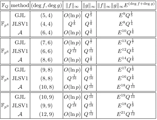
We compare the norm bounds for t = 2, i.e., when the sieving polynomial is linear. In this case, Table 2 lists the degrees and norm bounds of polynomials for various methods. Table 3 compares the new method with the JLSV1 and the GJL method for concrete values ofn,randd. This shows that the new method provides different trade-offs which were not known earlier.
As an example, we can see from Table 3 that the new method compares well with GJL and JLSV1 methods for n = 4 and Qof 300 dd (refer to Table 1). As mentioned in [5], when the differences between the methods are small, it is not possible to decide by looking only at the size of the norm product. Keeping this in view, we see that the new method is competitive forn= 6 as well. These observations are clearly visible in the plots given in the Figure 3. From the Q
-E pairs given in Table 1, it is clear that the increase ofE is slower than that of Q. This suggests that the new method will become competitive when Q is sufficiently large.
Next we provide some concrete examples of polynomialsf(x), g(x) andϕ(x) obtained using the new method. The examples are for n = 6 andn = 4. For
n = 6, we have taken d = 1,2,3 and 6 and in each case r was chosen to be
r=k=n/d. Forn= 4, we considerd= 2 withr=k=n/dandr=k+ 1; and
(a) Polynomials forFp4 (b) Polynomials forFp6
Fig. 3.Product of norms for various polynomial selection methods
Table 2.Parameterised efficiency estimates for NFS obtained from the different poly-nomial selection methods.
Methods degf degg kfk∞ kgk∞ kfk∞kgk∞E(degf+degg)
JLSV1 n n Q21n Q21n E2nQ1n
GJL (r≥n) r+ 1 r O(lnp) Qr+11 E2r+1Q 1
r+1
Conjugation 2n n O(lnp) Q21n E3nQ21n
A(d|n,r≥n/d)d(r+ 1) dr O(lnp)Qd(r1+1) Ed(2r+1)Q1/(d(r+1))
Table 3.Comparison of efficiency estimates for compositenwithd= 2 andr=n/2.
FQ method (degf,degg) kfk∞ kgk∞kfk∞kgk∞E(degf+degg)
Fp4
GJL (5,4) O(lnp) Q15 E9Q 1 5
JLSV1 (4,4) Q18 Q18 E8Q14
A (6,4) O(lnp) Q16 E10Q 1 6
Fp6
GJL (7,6) O(lnp) Q17 E13Q 1 7
JLSV1 (6,6) Q121 Q121 E12Q16
A (8,6) O(lnp) Q18 E14Q18
Fp8
GJL (9,8) O(lnp) Q19 E17Q19
JLSV1 (8,8) Q161 Q 1
16 E16Q 1 8
A (10,8) O(lnp) Q101 E18Q101
Fp9
GJL (10,9) O(lnp) Q101 E19Q101
JLSV1 (9,9) Q181 Q181 E18Q19
A (12,9) O(lnp) Q121 E21Q 1 12
Example 1. Letn= 6, and pis a 201-bit prime given below.
Takingd= 1 andr=n/d, we get
f(x) =x7+18x6+99x5−107x4−3470x3−15630x2−30664x−23239
g(x) =712965136783466122384156554261504665235609243446869x6+16048203858903 260691766216702652575435281807544247712x5+14867720774814154920358989 0852868028274077107624860184x4+7240853845391439257955648357229262561 71920852986660372x3+194693204195493982969795038496468458378024972218 5345772x2+2718971797270235171234259793142851416923331519178675874x +1517248296800681060244076172658712224507653769252953211
ϕ(x) =x6+671560075936012275401828950369729286806144005939695349290760x5+ 774705834624554066737199160555511502088270323481268337340514x4+1100 646447552671580437963861085020431145126151057937318479717x3+27131646 3864123658232870095113273120009266491174096472632727x2+4101717389506 73951225351009256251353058695601874372080573092x+1326632804961027767 272334662693578855845363854398231524390607
Note thatkgk∞≈2180. Takingd= 2 andr=n/d, we get
f(x) =x8−x7−5x6−50x5−181x4−442x3−801x2−633x−787
g(x) =833480932500516492505935839185008193696457787x6+2092593616641287655 065740032896986343580698615x5+1298540899568952261791537743468335194 3188533320x4+21869741590966357897620167461539967141532970622x3+6 4403097224634262677273803471992671747860968564x2+558647116952815842 83909455665521092749502793807x+921778354059077827252784356704871327 10722661831
ϕ(x) =x6+225577566898041285405539226183221508226286589225546142714057x5+ 726156673723889082895351451739733545328394720523246272955173x4+10214 78132054694721578888994001730764934454660630543688348056x3+674978102 55620874288201802771995130845407860934811815878391x2+632426210761786 622105494194314937817927439372918029042718843x+104093530686601670252 6455143725415379604742339065421793844038
Note thatkgk∞≈2156. Takingd= 3 andr=n/d, we get
g(x) =2889742364508381557593312392497801006712x6+83633695370646306085610 87765146274738509x5+10828078806524085705506412783408772941877x4+ 41812824889730400169000397417267197701179x3+1497421347777532476213 31508897969482387354x2+240946716989443210293442965552611305592194x +151696455655104744403073743333940426598833
ϕ(x) =x6+265074577705978624915342871970538348132010154368109244143774x5 +21159801273629654486978970226092134077566675973129512551886x4+10 63445611445684266941289540827947199397416276334188055837892x3+1459 587283058054365639950761731919998074021438242745336103973x2+145654 3437800571643325638648207188371117923539168263210522995x+378129170 960510211491600303623674471468414144797178846977007
Note thatkgk∞≈2137. Takingd= 6 andr=n/d, we get
f(x) =x12+3x10+10x9+53x8+112x7+163x6 +184x5+177x4+166x3+103x2+72x+48
g(x) =−666878138402353195498832669848x6−1867253271074924746011849188889x5 −5601759813224774238035547566667x4−6668753801765210948063915265053x3 −4268003536420067847037882226971x2−6935516090029480629033212906363x −7469013084299698984047396755556
ϕ(x) =x6+356485336847074091920944597187811284411849047991334266185684x5+ 1069456010541222275762833791563433853235547143974002798557052x4+175 488639976380184062760893597893819537042246173878495567205x3+1069456 010541222275762833791563433853235547143974002798557050x2+1069456010 541222275762833791563433853235547143974002798557054x+14259413473882 96367683778388751245137647396191965337064742736
In this case we get kgk∞≈2102.
Example 2. Letn= 4, and pis a 301-bit prime given below.
p=203703597633448608626844568840937816105146839366593625063614044935438 1299763336706183493607
Takingd= 2 andr=n/d, we get
g(x) =1108486244023576208689360410176300373132220654590976786482134x4+20 50762938144982289360096083705563965935573667103554994528044x3+5523 467580377021934753091786207648479867036209679151793015319x2+456222 7246514756745388645848004531501269616133890841445574058x+441498133 6353445726063731376031348106734815555088175006533185
ϕ(x) =x4+1305623360698284685175599277707343457576279146188242586245210199 344777856138293049165536292x3+1630663764713242722426772175575945319 640665655794962932653634545690570677252853972689997048x2+1955704168 7282007596779450734445471817050521654016832790620588920363634983674148
96214457800x+163066376471324272242677217557594531964066565579496293 2653634545690570677252853972689997047
In this case we havekgk∞≈2201. If we take r=n/d+ 1, we get
f(x) =x8+16x7+108x6+398x5+865x4+1106x3+820x2+328x+55
g(x) =348482147842083865380881347784399925335728557x6+5536103979982210590 186016445459289773029045618x5+3381254505070666477453052572333514580 1290667783x4+96062171957261124763428590648958745188735445330x3+1 24085795781307363759935898131887563792535489069x2+73090839973729169 966964061428402316131911130808x+16093810783274309055350481972028841 649178007790
ϕ(x) =x4+5128690964597943246501962358998676237033930846168967447990334244 55696319185673262765599428x3+1802408796932749487444974790576022081 708344659229207911271845827650035713383268427662416444x2+1553341208 0263216762891646375525736686031169799908288433475579574772861500238438
04262435184x+263801507553366513494386082876419210598165405378517676 874745554282946755826248639365618168
In this case we havekgk∞≈2156. If we take d= 4 andr=d/n, we have
f(x) =x8−3x7−33x6−97x5−101x4+3x3+73x2−35x−8
ϕ(x) =x4+3001292991290566658187708046113162326822746963576576248059013380 7217067092452460559896554x3+900387897387169997456312413833948698046 82408907297287441770401421651201277357381679689656x2+15006464956452 8332909385402305658116341137348178828812402950669036085335462262302799
482756x+30012929912905666581877080461131623268227469635765762480590 133807217067092452460559896553
In this case also we havekgk∞≈2150.
7
Asymptotic Complexity Analysis
The goal of the asymptotic complexity analysis is to express the runtime of the NFS algorithm using the L-notation and at the same time obtain bounds onp
for which the analysis is valid. Our description of the analysis is based on prior works predominantly those in [17, 19, 5, 24].
For 0< a <1, write
p=LQ(a, cp), where cp= 1
n
lnQ
ln lnQ 1−a
and so n= 1
cp
lnQ
ln lnQ 1−a
.
(15)
The value of a will be determined later. Also, for each cp, the runtime of the NFS algorithm is the same for the family of finite fields Fpn where p is given
by (15).
From Section 3, we recall the following.
1. The number of polynomials to be considered for sieving isE2. 2. The factor base is of size B.
Sparse linear algebra using the Lanczos or the block Wiedemann algorithm takes timeO(B2). For some 0< b <1, let
B=LQ(b, cb). (16)
The value ofb will be determined later. Set
E=B (17)
so that asymptotically, the number of sieving polynomials is equal to the time for the linear algebra step.
Letπ= Ψ(Γ, B) be the probability that a random positive integer which is at most Γ isB-smooth. Let Γ =LQ(z, ζ) andB=LQ(b, cb). Using the L-notation version of the Canfield-Erd¨os-Pomerance theorem,
(Ψ(Γ, B))−1=LQ
z−b,(z−b)ζ
cb
The bound on the product of the norms given by Proposition 2 is
Γ =E2td(2r+1)×Q t−1
d(r+1). (19)
Note that in (19), t−1 is the degree of the sieving polynomial. Following the usual convention, we assume that the same smoothness probability πholds for the event that a random sieving polynomialφ(x) is smooth over the factor base. The expected number of polynomials to consider for obtaining one relation is
π−1. Since B relations are required, obtaining this number of relations requires trying Bπ−1 trials. Balancing the cost of sieving and the linear algebra steps requiresBπ−1=B2and so
π−1=B. (20)
Obtainingπ−1 from (18) and setting it to be equal to B allows solving for c b. Balancing the costs of the sieving and the linear algebra phases leads to the runtime of the NFS algorithm to be B2 = LQ(b,2cb). So, to determine the runtime, we need to determine band cb. The value of bwill turn out to be 1/3 and the only real issue is the value ofcb.
Lemma 1. Let n=kdfor positive integers k andd. Using the expressions for
pandE(=B)given by (15) and (16), we obtain the following.
E2td(2r+1)=LQ
1−a+b,2cb(2r+1)
cpkt
;
Qd(tr−+1)1 =L
Q
a,kcp(t−1)
(r+1) . (21)
Proof. The second expression follows directly from Q=pn, p=LQ(a, cp) and
n=kd. The computation for obtaining the first expression is the following.
E2td(2r+1)=LQ
b, cb 2
td(2r+ 1)
= exp
cb
2
t(2r+ 1) n k(lnQ)
b(ln lnQ)1−b
= exp cb 2
cpkt
(2r+ 1)
lnQ
ln lnQ 1−a
(lnQ)b(ln lnQ)1−b
!
=LQ
1−a+b,2cb(2r+ 1) cpkt
.
u t
Theorem 1 (Boundary Case). Let k divide n, r ≥ k, t ≥ 2 and p =
LQ(2/3, cp)for some0< cp<1. It is possible to ensure that the runtime of the
NFS algorithm with polynomials chosen by AlgorithmAisLQ(1/3,2cb)where
cb= 2r+ 1
3cpkt +
s
2r+ 1
3cpkt
2
+kcp(t−1)
Proof. Setting 2a= 1 +b, the two L-expressions given by (21) have the same first component and so the product of the norms is
Γ =LQ
a,2cb(2r+ 1) cpkt
+kcp(t−1) (r+ 1)
.
Thenπ−1given by (18) is
LQ
a−b,(a−b)
2(2r+ 1) cpkt
+kcp(t−1)
cb(r+ 1)
.
From the conditionπ−1=B, we getb=a−b and
cb = (a−b)
2(2r+ 1) cpkt
+kcp(t−1)
cb(r+ 1)
.
The conditionsa−b =b and 2a= 1 +b show that b= 1/3 anda= 2/3. The second equation then becomes
cb= 1 3
2(2r+ 1) cpkt
+kcp(t−1)
cb(r+ 1)
. (23)
Solving the quadratic forcb and choosing the positive root gives
cb= 2r+ 1
3cpkt +
s
2r+ 1
3cpkt
2
+kcp(t−1) 3(r+ 1) .
u t
Corollary 1 (Boundary Case of the Conjugation Method [5]). Let r=
k= 1. Then forp=LQ(2/3, cp), the runtime of the NFS algorithm isLQ(1/3,2cb)
with
cb = 1
cpt +
s
1
cpt
2
+cp(t−1)
6 .
Allowing r to be greater than k leads to improved asymptotic complexity. We do not perform this analysis. Instead, we perform the analysis in the similar situation which arises for the multiple number field sieve algorithm.
Theorem 2 (Medium Characteristic Case). Let p = LQ(a, cp) with a >
1/3. It is possible to ensure that the runtime of the NFS algorithm with the polynomials produced by AlgorithmAisLQ(1/3,(32/3)1/3).
Proof. Since a >1/3, the bound Γ on the product of the norms can be taken to be the expression given by (7). The parameter tis chosen as follows [5]. For 0 < c < 1, let t = ctn((lnQ)/(ln lnQ))−c. For the asymptotic analysis, t−1 is also assumed to be given by the same expression for t. Then the expressions given by (21) become the following.
E2td(2r+1)=LQ
b+c,2cb(2r+1)
kct
; Qd(tr−+1)1 =L
Q
1−c, kct
r+1
This can be seen by substituting the expression fortin (21) and further by using the expression forngiven in (15).
Setting 2c= 1−b, the first components of the two expressions in (24) become equal and so
Γ =LQ
b+c,2cb(2r+ 1) kct
+ kct
r+ 1
.
Using this Γ, the expression forπ−1is
π−1=LQ
c, c
2(2r+ 1)
kct
+ kct
cb(r+ 1)
.
We wish to choosectso as to maximise the probabilityπand hence to minimise
π−1. This is done by setting 2(2r+ 1)/(kc
t) = (kct)/(cb(r+ 1)) whence kct=
p
2cb(r+ 1)(2r+ 1). With this value ofkct,
π−1=LQ c,
2cp2cb(r+ 1)(2r+ 1)
cb(r+ 1)
!
.
Setting π−1 to be equal toB=LQ(b, cb) yieldsb=cand
cb=
2cp2cb(r+ 1)(2r+ 1)
cb(r+ 1)
!
.
From b=c and 2c= 1−b we obtainc=b= 1/3. Using this value ofc in the equation forcb, we obtaincb= (2/3)2/3×((2(2r+ 1))/(r+ 1))1/3. The value of
cb is the minimum forr= 1 and this value iscb= (4/3)1/3. ut Note that the parameterawhich determines the size ofpis not involved in any of the computation. The assumptiona >1/3 is required to ensure that the bound on the product of the norms can be taken to be the expression given by (7). Theorem 3 (Large Characteristic). It is possible to ensure that the run-time of the NFS algorithm with the polynomials produced by Algorithm A is
LQ(1/3,(64/9)1/3)forp≥LQ(2/3,(8/3)1/3).
Proof. Following [5], for 0 < e < 1, let r = cr/2((lnQ)/(ln lnQ))e. For the asymptotic analysis, the expression for 2r+ 1 is taken to be two times this expression. Substituting this expression forrin (21), we obtain
E2td(2r+1)=LQ
1−a+b+e,2cbcr
cpkt
;
Qd(tr−+1)1 =L
Q
a−e,2kcp(t−1)
cr . (25)
Setting 1 +b = 2(a−e), we obtain Γ =LQ
1 +b
2 , 2cbcr
cpkt
+2kcp(t−1)
cr
and so the probabilityπ−1 is given by
LQ
1−b
2 , 1−b
2 ×
2c
r
cpkt
+2kcp(t−1)
crcb
The choice of cr for which the probability π is maximised (and hence π−1 is minimised) is obtained by setting cr/(cpk) =
p
(t(t−1))/cb and the minimum value ofπ−1 is
LQ
1−b
2 , 1−b
2 ×
4
r t−1
tcb
.
Setting this value ofπ−1to be equal to B, we obtain
b= (1−b)/2; cb= 1−b
2 ×
4
r t−1
tcb
.
The first equation showsb= 1/3 and using this in the second equation, we obtain
cb= (4/3)2/3((t−1)/t)1/3. This value ofcb is minimised for the minimum value oft which ist= 2. This givescb = (8/9)1/3.
Using 2(a−e) = 1 +bandb= 1/3 we geta−e= 2/3. Note thatr≥kand so p≥pk/r =LQ(a,(c
pk)/r) =LQ(a−e,(2cpk)/cr). With t= 2, the value of (cpk)/cr is equal to (1/3)1/3and so p≥LQ(2/3,(8/3)1/3). ut Theorems 2 and 3 show that the generality introduced byk and r do not affect the overall asymptotic complexity for the medium and large prime case and the attained complexities in these cases are the same as those obtained for previous methods in [5].
8
Multiple Number Field Sieve Variant
As the name indicates, the multiple number field sieve variant uses several num-ber fields. The discussion and the analysis will follow the works [8, 24].
There are two variants of multiple number field sieve algorithm. In the first variant, the image ofφ(x) needs to be smooth in at least any two of the number fields. In the second variant, the image of φ(x) needs to be smooth in the first number field and at least one of the other number fields.
We have analysed both the variants of multiple number field sieve algorithm and found that the second variant turns out to be better than the first one. So we discuss the second variant of MNFS only. In contrast to the number field sieve algorithm, the right number field is replaced by a collection ofV number fields in the second variant of MNFS. The sieving polynomialφ(x) has to satisfy the smoothness condition on the left number field as before. On the right side, it is sufficient for φ(x) to satisfy a smoothness condition on at least one of the
V number fields.
Recall that AlgorithmAproduces two polynomialsf(x) andg(x) of degrees
d(r+1) anddrrespectively. The polynomialg(x) is defined as Resy(ψ(y), C0(x)+
yC1(x)) whereψ(x) = LLL(MA2,r), i.e.,ψ(x) is defined from the first row of the
matrix obtained after applying the LLL-algorithm toMA2,r.
from the second row of the matrixMA2,r. Define g1(x) = Resy(ψ1(y), C0(x) +
yC1(x)) and g2(x) = Resy(ψ2(y), C0(x) +yC1(x)). Then choose V −2 linear combinationsgi(x) =sig1(x)+tig2(x), fori= 3, . . . , V. Note that the coefficients
si and ti are of the size of √
V. All the gi’s have degree dr. Asymptotically, kψ2k∞ = kψ1k∞ =Q1/(d(r+1)). Since we take V = LQ(1/3), all the gi’s have their infinity norms to be the same as that ofg(x) given by Proposition 2.
For the left number field, as before, letB be the bound on the norms of the ideals which are in the factor basis defined by f. For each of the right number fields, let B0 be the bound on the norms of the ideals which are in the factor basis defined by each of thegi’s. So, the size of the entire factor basis isB+V B0. The following condition balances the left portion and the right portion of the factor basis.
B =V B0. (26)
With this condition, the size of the factor basis is B1+o(1) as in the classical NFS and so asymptotically, the linear algebra step takes timeB2. As before, the number of sieving polynomials is E2=B2 and the coefficients ofφ(x) can take
E2/tdistinct values.
Letπ be the probability that a random sieving polynomialφ(x) gives rise to a relation. Let π1 be the probability thatφ(x) is smooth over the left factor basis and π2 be the probability that φ(x) is smooth over at least one of the right factor bases. Further, let Γ1= Resx(f(x), φ(x)) be the bound on the norm corresponding to the left number field and Γ2= Resx(gi(x), φ(x)) be the bound on the norm for any of the right number fields. Note that Γ2 is determined only by the degree and the L∞-norm of gi(x) and hence is the same for all gi(x)’s. Heuristically, we have
π1= Ψ(Γ1, B);
π2=VΨ(Γ2, B0);
π=π1×π2.
(27)
As before, one relation is obtained in about π−1 trials and so B relations are obtained in aboutBπ−1trials. Balancing the cost of linear algebra and sieving, we have as beforeB=π−1.
The following choices ofB andV are made.
E=B=LQ 13, cb;
V =LQ 13, cv; and so
B0=B/V =LQ 13, cb−cv.
(28)
With these choices ofB and V, it is possible to analyse the MNFS variant for AlgorithmAfor three cases, namely, the medium prime case, the boundary case and the large characteristic case. Below we present the details of the boundary case. This presents a new asymptotic result.
Theorem 4 (MNFS-Boundary Case). Let kdivide n,r≥k,t≥2 and
p=LQ
2
3, cp
where cp= 1
n
lnQ
ln lnQ 1/3
It is possible to ensure that the runtime of the MNFS algorithm is LQ(1/3,2cb)
where
cb= 4r+ 2
6ktcp +
s
r(3r+ 2) (3ktcp)2 +
cpk(t−1)
3(r+ 1) . (29)
Proof. Note the following computations. Γ1=kφkdeg(f)
∞ =E2deg(f)/t=E(2d(r+1))/t=E(2n(r+1))/(kt) =LQ
2
3,
2(r+ 1)cb
ktcp
;
π−11=LQ
1 3,
2(r+ 1) 3ktcp
;
Γ2=kφkdeg(g)∞ × kgkdeg(φ)∞ =E2deg(g)/t×Q(t−1)/(d(r+1)) =E(2rd)/t×Q(t−1)/(d(r+1))=E(2rn)/(kt)×Qk(t−1)/(n(r+1))
=LQ
2
3, 2rcb
cpkt
+kcp(t−1)
r+ 1
;
π−21=LQ
1
3,−cv+ 1 3(cb−cv)
2rc
b
cpkt
+kcp(t−1)
r+ 1
;
π−1=LQ
1
3,
2(r+ 1) 3ktcp
−cv+ 1 3(cb−cv)
2rc
b
cpkt
+kcp(t−1)
r+ 1
;
From the conditionπ−1=B, we obtain the following equation.
cb =
2(r+ 1) 3ktcp
−cv+ 1 3(cb−cv)
2rc
b
cpkt
+kcp(t−1)
r+ 1
. (30)
We wish to findcvsuch thatcbis minimised subject to the constraint (30). Using the method of Lagrange multipliers, the partial derivative of (30) with respect tocv gives
cv=
r+ 1 3ktcp
.
Using this value ofcv in (30) provides the following quadratic in cb.
(3ktcp)c2b−(4r+ 2)cb+
(r+ 1)2 3ktcp
−(cpk)
2t(t−1)
r+ 1 = 0.
Solving this and taking the positive square root, we obtain
cb= 4r+ 2
6ktcp +
s
r(3r+ 2) (3ktcp)2
+cpk(t−1)
3(r+ 1) . (31)
8.1 Further Analysis of the Boundary Case
Theorem 4 expresses 2cb as a function of cp, t, k and r. Let us write this as 2cb = C(cp, t, k, r). It turns out that fixing the values of (t, k, r) gives a set
S(t, k, r) such that for cp ∈ S(t, k, r), C(cp, t, k, r) ≤ C(cp, t0, k0, r0) for any (t0, k0, r0) 6= (t, k, r). In other words, for a choice of (t, k, r), there is a set of values for cp where the minimum complexity of MNFS-A is attained. The set
S(t, k, r) could be empty implying that the particular choice of (t, k, r) is sub-optimal.
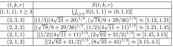
For 1.12 ≤ cp ≤ 4.5, the appropriate intervals are given in Table 4. Fur-ther, the interval (0,1.12] is the union of S(t,1,1) for t ≥ 3. Note that the choice (t, k, r) = (t,1,1) specialises MNFS-A to MNFS-Conjugation. So, for
cp ∈ (0,1.12]∪[1.45,3.15] the complexity of MNFS-A is the same as that of MNFS-Conjugation.
Table 4.Choices of (t, k, r) and the correspondingS(t, k, r).
(t, k, r) S(t, k, r)
(t,1,1),t≥3 S
t≥3S(t,1,1)≈(0,1.12]
(2,3,3) [(1/3)(4√21 + 20)1/3,(√78/9 + 29/36)1/3]≈[1.12,1.21] (2,2,2) [(√78/9 + 29/36)1/3,(1/2)(4√11 + 11)1/3]≈[1.21,1.45] (2,1,1) [(1/2)(4√11 + 11)1/3,(2√62 + 31/2)1/3]≈[1.45,3.15] (2,1,2) [(2√62 + 31/2)1/3,(8√33 + 45)1/3]≈[3.15,4.5]
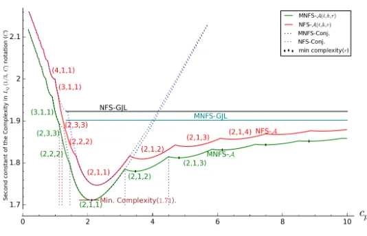
In Figure 4, we have plotted 2cb given by Theorem 4 against cp for some values oft,kandrwhere the minimum complexity of MNFS-Ais attained. The plot is labelled MNFS-A. The setsS(t, k, r) are clearly identifiable from the plot. The figure also shows a similar plot for NFS-A which shows the complexity in the boundary case given by Theorem 1. For comparison, we have plotted the complexities of the GJL and the Conjugation methods from [5] and the MNFS-GJL and the MNFS-Conjugation methods from [24].
Based on the plots given in Figure 4, we have the following observations. 1. Complexities of NFS-Aare never worse than the complexities of NFS-GJL
and NFS-Conjugation. Similarly, complexities of MNFS-Aare never worse than the complexities of MNFS-GJL and MNFS-Conjugation.
2. For both the NFS-A and the MNFS-A methods, increasing the value of r
provides new complexity trade-offs.
3. There is a value of cp for which the minimum complexity is achieved. This corresponds to the MNFS-Conjugation. LetLQ(1/3, θ0) be this complexity. The value ofθ0 is determined later.
5. For smaller values ofcp, it is advantageous to chooset >2 ork >1. On the other hand, for larger values ofcp, the minimum complexity is attained for
t= 2 andk= 1.
Fig. 4.Complexity plot for boundary case
From the plot, it can be seen that for larger values ofcp, the minimum value ofcbis attained fort= 2 andk= 1. So, we decided to perform further analysis using these values oftandk.
8.2 Analysis for t= 2 andk= 1
Fixt= 2 andk= 1 and let us denoteC(cp,2,1, r) as simplyC(cp, r). Then from Theorem 4 the complexity of MNFS-A forp=LQ(2/3, cp) is LQ(1/3,C(cp, r)) where
C(cp, r) = 2cb = 2
s cp 3 (r+ 1) +
(3r+ 2)r
36c2 p
+2r+ 1 3cp
. (32)
Figure 4 shows that for each r≥1, there is an interval [0(r), 1(r)] such that forcp ∈[0(r), 1(r)],C(cp, r)<C(cp, r0) forr6=r0. Forr= 1, we have
0(1) = 1 2
4√11 + 11
1 3
≈1.45; 1(1) =
2√62 +31 2
13
≈3.15.
lower than the complexity of all prior methods. The following result shows that the minimum complexity attainable by MNFS-Aapproaches the complexity of MNFS-GJL from below.
Theorem 5. Forr≥1, letC(r) = mincp>0C(cp, r). Then
1. C(1) =θ0= 146261 √
22 +208871/3.
2. Forr≥1,C(r)is monotone increasing and bounded above. 3. The limiting upper bound ofC(r)isθ1=
2×(13√13+46)
27
1/3 .
Proof. DifferentiatingC(cp, r) with respect tocpand equating to 0 gives
6 r+1−
(3r+2)r c3
p
18q cp
3 (r+1)+ (3r+2)r
36c2
p
−2r+ 1 3c2
p
= 0 (33)
On simplifying we get, 6c3
p−(3r+ 2)r(r+ 1)
r
12c3
p+ (r+ 1)(3r+ 2)r
(r+ 1)
−2r+ 1
1 = 0 (34)
Equation (34) is quadratic in c3
p. On solving we get the following value ofcp.
cp=
7
6r 3+13
6 r 2+1
6
p
13r2+ 10r+ 1 2r2+ 3r+ 1
+7 6r+
1 6
1/3
‡
=ρ(r) (say). (35)
Putting the value of cp back in (32), we get the minimum value of C (in terms ofr) as
C(r) = 2
s ρ(r) 3 (r+ 1)+
(3r+ 2)r
36ρ(r)2 + 2r+ 1
3ρ(r). (36)
All the three sequences in the expression for C(r), viz, 3 (r+1)ρ(r) , (336r+2)rρ(r)2 and
2r+1
3ρ(r) are monotonic increasing. This can be verified through computation (with a symbolic algebra package) as follows. Let sr be any one of these sequences. Then computing sr+1/sr gives a ratio of polynomial expressions from which it is possible to directly argue that sr+1/sr is greater than one. We have done these computations but, do not present the details since they are uninteresting and quite messy. Since all the three sequences 3 (r+1)ρ(r) , (336r+2)rρ(r)2 and
2r+1 3ρ(r) are monotonic increasing so isC(r).
‡
Note that forr≥1,ρ(r)>(7/6)1/3r >1.05r. So, forr >1, (3r+ 2)r
ρ(r)2 = 3
r ρ(r)
2
+ 2 r
ρ(r)2 <3×
1 1.05
2
+ 2× 1 1.05. (2r+ 1)
ρ(r) = 2
r ρ(r)+
1
ρ(r) <2× 1 1.05+
1 1.05. This shows that the sequences (3r+2)rρ(r)2 and
(2r+1)
ρ(r) are bounded above. Forr >8, we have (3r+1)<(8r+1)< r2and (2r2+r+1/6)< r3/3 which implies that for
r >8,ρ(r)<(7/6+1/6×√14×3+1/3)1/3r <1.5r. Usingρ(r)<1.5rforr >8, it can be shown that the sequence ρ(r)r+1
r>8
is bounded above by 1.5. Since the three constituent sequences (r+1)ρ(r) , (3ρ(r)r+2)r2 and
2r+1
ρ(r) are bounded above, it follows thatC(r) is also bounded above. Being monotone increasing and bounded aboveC(r) is convergent. We claim that
lim
r→∞C(r) =
2×(13√13 + 46) 27
!1/3 .
The proof of the claim is the following. Using the expression forρ(r) from (35) we have lim
r→∞
ρ(r)
r =
2
6 √
13 +7 6
13
. Now,
C(r) = 2
s
ρ(r)/r
3 (1 + 1/r)+
(3 + 2/r) 36ρ(r)2/r2 +
2 + 1/r
3ρ(r)/r. (37)
Hence,
lim
r→∞C(r) = 2
s
(2√13 + 7)1/3 3×61/3 +
3×62/3 36 (2√13 + 7)2/3 +
2×61/3 3 (2√13 + 7)1/3
After further simplification, we get
lim
r→∞C(r) =
2×(13√13 + 46) 27
!1/3 .
The limit ofC(r) asrgoes to infinity is the value ofθ1whereLQ(1/3, θ1) is the complexity of MNFS-GJL as determined in [24]. This shows that as r goes to infinity, the complexity of MNFS-A approaches the complexity of MNFS-GJL from below.
We have already seen that C(r) is monotone increasing for r ≥1. So, the minimum value ofC(r) is obtained forr= 1. After simplifyingC(1), we get the minimum complexity of MNFS-Ato be
LQ
1/3,
3 +
q
3(11 + 4√6) 18 7 + 3√61/3
This minimum complexity is obtained atcp=ρ(1) = 2 √
6 +14313 = 2.123 .§ u t
Note 1. As mentioned earlier, forr=k= 1, the new method of polynomial selec-tion becomes the Conjugaselec-tion method. So, the minimum complexity of MNFS-A is the same as the minimum complexity for MNFS-Conjugation. Here we note that the value of the minimum complexity given by (38), is not same as the one reported by Pierrot in [24]. This is due to an error in the calculation in [24]¶.
Complexity of NFS-A: From Figure 4, it can be seen that there is an interval forcpfor which the complexity of NFS-Ais better than both MNFS-Conjugation and MNFS-GJL. An analysis along the lines as done above can be carried out to formally show this. We skip the details since these are very similar to (actually a bit simpler than) the analysis done for MNFS-A. Here we simply mention the following two results:
1. Forcp≥ 2 √
89 + 2013 ≈3.39, the complexity of NFS-Ais better than that
of MNFS-Conjugation. 2. Forcp≤ 18
√ 390
q
5√13−18 2627√13 +9227
1 3+45
8 26 27
√
13 +9227
2
3 ≈20.91,
the complexity of NFS-Ais better than that of MNFS-GJL.
3. So, for cp ∈[3.39,20.91], the complexity of NFS-Ais better than the com-plexity of all previous method including the MNFS variants.
Current state-of-the-art: The complexity of MNFS-Ais lower than that of NFS-A. As mentioned earlier (before Table 4) the interval (0,1.12] is the union of ∪t≥3S(t,1,1). This fact combined with Theorem 5 and Table 4 show the following. Forp=LQ(2/3, cp), whencp∈(0,1.12]∪[1.45,3.15], the complexity of MNFS-Ais the same as that of MNFS-Conjugation; forcp∈/(0,1.12]∪[1.45,3.15] and cp >0, the complexity of MNFS-Ais smaller than all previous methods. Hence, MNFS-A should be considered to provide the current state-of-the-art asymptotic complexity in the boundary case.
8.3 Medium and Large Characteristic Cases
In a manner similar to that used to prove Theorem 4, it is possible to work out the complexities for the medium and large characteristic cases of the MNFS corresponding to the new polynomial selection method. To tackle the medium prime case, the value oftis taken to bet=ctn((lnQ)(ln lnQ))−
1/3
and to tackle the large prime case, the value of r is taken to ber=cr/2 ((lnQ)(ln lnQ))1/3.
§
These values are incorrect in the proceedings version and the source of error was the incorrect expression for equation (35).
¶
The error is the following. The solution for cb to the quadratic (18t2c2p)c2b −
(36tcp)cb + 8 −3t2(t −1)c3
p = 0 is cb = 1/(tcp) + p
This will provide a relation betweencb, cv andr(for the medium prime case) or
t(for the large prime case). The method of Lagrange multipliers is then used to find the minimum value of cb. We have carried out these computations and the complexities turn out to be the same as those obtained in [24] for the MNFS-GJL (for large characteristic) and the MNFS-Conjugation (for medium characteristic) methods. Hence, we do not present these details.
9
Conclusion
In this work, we have proposed a new method for polynomial selection for the NFS algorithm for fieldsFpn withn >1. Asymptotic analysis of the complexity
has been carried out both for the classical NFS and the MNFS algorithms for polynomials obtained using the new method. For the boundary case with p=
LQ(2/3, cp) forcpoutside a small set, the new method provides complexity which is lower than all previously known methods.
References
1. Leonard M. Adleman. The function field sieve. In Leonard M. Adleman and Ming-Deh A. Huang, editors,ANTS, volume 877 ofLecture Notes in Computer Science, pages 108–121. Springer, 1994.
2. Leonard M. Adleman and Ming-Deh A. Huang. Function field sieve method for discrete logarithms over finite fields. Inf. Comput., 151(1-2):5–16, 1999.
3. Shi Bai, Cyril Bouvier, Alain Filbois, Pierrick Gaudry, Laurent Imbert, Alexander Kruppa, Fran¸cois Morain, Emmanuel Thom´e, and Paul Zimmermann. CADO-NFS, an implementation of the number field sieve algorithm. CADO-CADO-NFS, Release 2.1.1, 2014. http://cado-nfs.gforge.inria.fr/.
4. Razvan Barbulescu. An appendix for a recent paper of Kim. IACR Cryptology ePrint Archive, 2015:1076, 2015.
5. Razvan Barbulescu, Pierrick Gaudry, Aurore Guillevic, and Fran¸cois Morain. Im-proving NFS for the discrete logarithm problem in non-prime finite fields. In Elisabeth Oswald and Marc Fischlin, editors, Advances in Cryptology – EURO-CRYPT 2015, volume 9056 ofLecture Notes in Computer Science, pages 129–155. Springer Berlin Heidelberg, 2015.
6. Razvan Barbulescu, Pierrick Gaudry, Antoine Joux, and Emmanuel Thom´e. A heuristic quasi-polynomial algorithm for discrete logarithm in finite fields of small characteristic. In Phong Q. Nguyen and Elisabeth Oswald, editors, Advances in Cryptology EUROCRYPT 2014, volume 8441 ofLecture Notes in Computer Sci-ence, pages 1–16. Springer Berlin Heidelberg, 2014.
7. Razvan Barbulescu, Pierrick Gaudry, and Thorsten Kleinjung. The tower number field sieve. In Tetsu Iwata and Jung Hee Cheon, editors, Advances in Cryptology – ASIACRYPT 2015, volume 9453 ofLecture Notes in Computer Science, pages 31–55. Springer, 2015.
9. Wieb Bosma, John Cannon, and Catherine Playoust. The Magma algebra system. I. The user language. J. Symbolic Comput., 24(3-4):235–265, 1997. Computational algebra and number theory (London, 1993).
10. Pierrick Gaudry, Laurent Grmy, and Marion Videau. Collecting relations for the number field sieve in GF(p6). Cryptology ePrint Archive, Report 2016/124, 2016.
http://eprint.iacr.org/.
11. Daniel M. Gordon. Discrete logarithms in GF(p) using the number field sieve.
SIAM J. Discrete Math, 6:124–138, 1993.
12. Robert Granger, Thorsten Kleinjung, and Jens Zumbr¨agel. Discrete logarithms in GF(29234). NMBRTHRY list, January 2014.
13. Aurore Guillevic. Computing individual discrete logarithms faster in GF(pn). Cryptology ePrint Archive, Report 2015/513, 2015. http://eprint.iacr.org/. 14. Antoine Joux. Faster index calculus for the medium prime case: Application to
1175-bit and 1425-bit finite fields. In Thomas Johansson and Phong Q. Nguyen, editors,EUROCRYPT, volume 7881 ofLecture Notes in Computer Science, pages 177–193. Springer, 2013.
15. Antoine Joux. A new index calculus algorithm with complexityL(1/4 +o(1)) in small characteristic. In Tanja Lange, Kristin E. Lauter, and Petr Lisonek, editors,
Selected Areas in Cryptography – SAC 2013, volume 8282 of Lecture Notes in Computer Science, pages 355–379. Springer, 2013.
16. Antoine Joux and Reynald Lercier. The function field sieve is quite special. In Claus Fieker and David R. Kohel, editors,ANTS, volume 2369 ofLecture Notes in Computer Science, pages 431–445. Springer, 2002.
17. Antoine Joux and Reynald Lercier. Improvements to the general number field sieve for discrete logarithms in prime fields. A comparison with the gaussian integer method. Math. Comput., 72(242):953–967, 2003.
18. Antoine Joux and Reynald Lercier. The function field sieve in the medium prime case. In Serge Vaudenay, editor,EUROCRYPT, volume 4004 ofLecture Notes in Computer Science, pages 254–270. Springer, 2006.
19. Antoine Joux, Reynald Lercier, Nigel P. Smart, and Frederik Vercauteren. The number field sieve in the medium prime case. In Cynthia Dwork, editor,Advances in Cryptology – CRYPTO, volume 4117 of Lecture Notes in Computer Science, pages 326–344. Springer, 2006.
20. Antoine Joux and C´ecile Pierrot. The special number field sieve in Fpn -
Ap-plication to pairing-friendly constructions. In Zhenfu Cao and Fangguo Zhang, editors,Pairing-Based Cryptography – Pairing 2013, volume 8365 ofLecture Notes in Computer Science, pages 45–61. Springer, 2013.
21. M. Kalkbrener. An upper bound on the number of monomials in determinants of sparse matrices with symbolic entries. Mathematica Pannonica, 8(1):73–82, 1997. 22. Taechan Kim. Extended tower number field sieve: A new complexity for medium
prime case. IACR Cryptology ePrint Archive, 2015:1027, 2015.
23. D. Matyukhin. Effective version of the number field sieve for discrete loga-rithm in a field GF(pk). Trudy po Discretnoi Matematike 9, 121151 (2006) (in Russian), 2006.http://m.mathnet.ru/php/archive.phtml?wshow=paper&jrnid= tdm&paperid=144&option_lang=eng.
24. C´ecile Pierrot. The multiple number field sieve with conjugation and generalized Joux-Lercier methods. In Advances in Cryptology – EUROCRYPT 2015, volume 9056 ofLecture Notes in Computer Science, pages 156–170, 2015.
26. Oliver Schirokauer. Discrete logarithms and local units. Philosophical Transac-tions: Physical Sciences and Engineering, 1993.
27. Oliver Schirokauer. Using number fields to compute logarithms in finite fields.
Math. Comp., 69(231):1267–1283, 2000.
28. Oliver Schirokauer. Virtual logarithms. J. Algorithms, 57(2):140–147, Nov 2005. 29. W. A. Stein et al.Sage Mathematics Software. The Sage Development Team, 2013.