Blackbox reduced-basis output bound methods for shape optimisation

45. A blackbox reduced-basis output bound method

for shape optimization

L. Machiels

_{, Y. Maday}

_{, A. T. Patera}

_{, D. V. Rovas}

Introduction

We present a two-stage off-line/on-line blackbox reduced-basis output bound method for the prediction of outputs of coercive partial differential equations with affine param-eter dependence. The computational complexity of the on-line stage of the procedure scales only with the dimension of the reduced-basis space and the parametric com-plexity of the partial differential operator. The method is both efficient and certain: thanks to rigorousa posteriorierror bounds, we may retain only the minimal number of modes necessary to achieve the prescribed accuracy in the output of interest. The technique is particularly appropriate for applications such as design and optimization, in which repeated and rapid evaluation of the output is required.

Reduced-basis methods [ASB78, Nag79, NP80] — projection onto low-order ap-proximation spaces comprising solutions of the problem of interest at selected points in the parameter/design space — are efficient techniques for the prediction of lin-ear functional outputs. These methods enjoy an optimality property which ensures rapid convergence even in high-dimensional parameter spaces; good accuracy is ob-tained even for very few modes (basis functions), and thus the computational cost is typically very small.

It is often the case that the parameter enters affinely in the differential operator. This allows us to separate the computational steps into two stages:(i) the off-line stage, in which the reduced-basis space is constructed; and (ii) theon-line/real time stage, in which for each new parameter value the reduced-basis approximation for the output of interest is calculated. The on-line stage is “blackbox” in the sense that there is no longer any reference to the original problem formulation:the computational complexity of this stage scales only with the dimension of the reduced-basis space and the parametric complexity of the partial differential operator.

Although a priori theory [FR83, Por85] suggests the optimality of the reduced-basis space approximation, for a particular choice of the reduced-reduced-basis space the error in the output of interest is typically not known, and hence the minimal number of basis functions required to satisfy the desired error tolerance can not be ascertained. As a result, either too many or too few basis functions are retained; the former results in computational inefficiency, the latter in uncertainty and unacceptably inaccurate

1_{Department of Mechanical Engineering, Massachusetts Institute of Technology, Room 3-264, 77}

Massachusetts Avenue, Cambridge, MA 01239, USA

2_{ASCI, UPR 9029, bˆatiment 506, Universit´e Paris-Sud, 91405 Orsay cedex, France; et Analyse}

num´erique, Universit´e Paris VI, 4, place Jussieu, 75252 Paris cedex 05, France

3_{Department of Mechanical Enginering, Massachusetts Institute of Technology, Room 3-264, 77}

Massachusetts Avenue, Cambridge, MA 01239, USA

4_{Department of Mechanical Engineering, Massachusetts Institute of Technology, Room 3-243, 77}

predictions. In this paper we develop blackboxa posteriorimethods that address these shortcomings. We consider here equilibrium solutions of coercive problems within the context of shape optimization; see also [MPR00] for treatment of noncoercive equilibrium problems and [MMO+00] for symmetric eigenvalue problems.

Numerical Method

Preliminaries

LetY be a Hilbert space with an associated inner product (·,·)_Y and an induced norm

· Y. We define our parameter space to beD ⊂R; a point in that space is denoted

µ. Our problem is then to findu∈Y such that

a(u, v;µ) =(v), ∀v∈Y, (1)

and subsequently the output of interest s(u) = 0(u); (·) and0(·) are both in Y, the dual space of Y. The bilinear form a is assumed to be continuous; symmetric,

a(w, v;µ) =a(v, w;µ), ∀w, v∈Y; and coercive,a(v, v;µ)≥cv2_Y >0, ∀v∈Y,∀µ∈

D, where c is a strictly positive real constant. Associated with the above primal problem we define the dual problem for ψ∈ Y : a(v, ψ;µ) =−0(v), ∀v ∈Y. The need for this problem will become clear in the error estimation discussion.

We next introduce a symmetric positive-definite form ˆa(w, v), and defineλ1_ˆa(µ) to be the minimum eigenvalue of a(ϕ, v;µ) =λ(µ)ˆa(ϕ, v), ∀v ∈Y. A lower bound for this eigenvalue is required by the output bound procedure:we assume that ag(µ) is known such that

a(v, v;µ)≥g(µ)ˆa(v, v)>0, ∀v∈Y and ∀µ∈ D. (2)

It is also possible to include approximation of λ1_aˆ(µ) as part of the reduced basis approximation [MPR00].

Finally, for the blackbox method, we shall assume that, for some finite integerQ, there exists a decomposition ofa(w, v;µ) of the form

a(w, v;µ) = Q

q=1

σq(µ)aq(w, v),∀w, v∈Yand∀µ∈ D, (3)

where we make no assumptions on theaq _{other than continuity and bilinearity.}

Reduced-Basis Approximation

We choose N/2 points in our parameter space D, and form the sample set

S_N = {µ₁, . . . , µ_N/2}. The reduced-basis spaces associated with the primal and dual problems are then given by W_Npr = span{u(µ₁), . . . , u(µ_N/2)} and W_Ndu = span{ψ(µ₁), . . . , ψ(µ_N/2)} respectively; we can now form

W_N = span{u(µ₁), ψ(µ₁), . . . , u(µ_N/2), ψ(µ_N/2)} ≡span{ζ₁, . . . , ζ_N}. (4)

For each new desired µ ∈ D, we now apply a standard Galerkin procedure over

W_N to obtain u_N(µ) andψ_N(µ) according to a(u_N(µ), v;µ) = (v), ∀v ∈ W_N, and

a(v, ψ_N(µ);µ) =−0(v), ∀v ∈W_N. The output can then be calculated ass_N(µ) =

0(u_N(µ)).

Bounds Evaluation

We start by defining the residuals associated with the primal and dual reduced-basis approximations,Rpr_{(v;µ) =(v)−a(u}

N(µ), v;µ), ∀v∈Y, andRdu(v;µ) =−0(v)−

a(v, ψ_N(µ);µ), ∀v∈Y, respectively. The Riesz representations ˆepr_{(µ) and ˆe}du_{(µ) of} the primal and dual residuals can then be defined as ˆa(ˆepr_{(µ), v) =R}pr_{(v;µ), ∀v ∈}

Y, aˆ(ˆedu_{(µ), v) =R}du_{(v;µ),∀v ∈Y.}

We then define, as in [MMO+00, MPR00],

¯

s_N(µ) = s_N(µ)− 1 2g(µ)ˆa(ˆe

pr_(µ),eˆdu_(µ)),

∆_N(µ) = 1 2g(µ)ˆa

1/2_(ˆepr_(µ),eˆpr_{(µ)) ˆa}1/2_(ˆedu_(µ),ˆedu_(µ)), (5)

and compute lower and upper estimatorss±_N = ¯s_N±∆_N.

It can be shown [MMO+00, MPR00] thats+_N (respectively s−_N) will be an upper (respectively lower) bound forsprovided thatg(µ) is a lower bound for the eigenvalue

λ1_ˆa(µ) (or equivalently satisfies (2)). Note that in the general case, where an ˆa and

g(µ) which satisfy (2) may not be readily available, the reduced-basis space must be augmented with eigenmodes corresponding to the minimum eigenvalue of the problem

a(ϕ, v;µ) =λ(µ)ˆa(ϕ, v), ∀v∈Y [MPR00].

Also of interest is the quality of the bounds — how well they approximate the actual error. We measure the quality of the bounds by the effectivityη_N(µ), defined as the ratio of the bound gap ∆_N to |s−s_N|. From the bound result we know that

η_N(µ)≥1. We can further prove [MPR00] thatη_N(µ) is bounded independent of N; in practice, η_N(µ) is typicallyO(1), as desired.

Blackbox Method

The parametric dependence assumed in (3) permits us to decouple the computation into two stages:the off-line stage, in which (i) the reduced basis is constructed and, (ii) the necessary error-estimation preprocessing is performed; and theon-line stage, in which for each new desired value ofµ, µ_d, we computes_N(µ_d) and the associated bounds. The essential “enabler” is the absence ofµdependence in ˆa, which allows us to precompute (and later assemble) all the “pieces” of ˆepr_(µ

d), and ˆedu(µd) by linear superposition. The details of the blackbox technique follow. For convenience we define

Off-line Stage

1. Calculateu(µ_i) andψ(µ_i), i= 1, . . . , N/2, to formW_N as in (4). 2. ComputeAq ∈RN×N _{as A}q

i,j=aq(ζi, ζj),∀i, j∈ N2 and∀q∈ Q.

3. Solve for ˆz0,pr _{∈Y and ˆz}0,du_{∈Y from ˆa(ˆz}0,pr_{, v) = (v), ∀v∈Y, and ˆa(ˆz}0,du_{, v) =}

−0(v), ∀v∈Y, respectively. Also, compute ˆz_jq∈Y from ˆa(ˆzq_j, v) =−aq_(ζ

j, v), ∀v∈

Y,∀j ∈ N and∀q∈ Q.

4. Calculate and store cpr₀ = ˆa(ˆz0,pr_,zˆ0,pr_{); c}du

0 = ˆa(ˆz0,du,zˆ0,du); cpr,du0 =

ˆ

a(ˆz0,pr_,zˆ0,du_{); F}pr

N,j = (ζj) and FN,jdu = 0(ζj), ∀j ∈ N; Λq,prj = ˆa(ˆz0,pr,zˆ q j) and Λ_jq,du= ˆa(ˆz0,du,zˆ_jq), ∀j∈ N and∀q∈ Q; Γpq_ij = ˆa(ˆz_ip,zˆ_jq),∀i, j∈ N2 and∀p, q∈ Q2. This stage requires (N Q+N+ 2)Y-linear system solves; (N2Q2+ 2N Q+ 3) ˆa-inner products; and 2N evaluations of linear functionals.

On-line Stage

For each new desired design point µ_d we then compute the reduced-basis prediction and error bound based on the quantities computed in the off-line stage.

1. FormA_N =Q_q=1σq_(µ

d)Aqand solve foruN ≡uN(µd)∈RN andψ_N ≡ψ_N(µd)∈

RN _fromA

N uN =FprN andAN ψ_N =−FduN, respectively. 2. Evaluate the bound average and bound gap as

¯

s_N = (Fdu_N)Tu_N−

1 2g(µ_d)(

N i=1 N j=1 Q p=1 Q q=1

u_N,iψ_N,jσp(µ_d)σq(µ_d)Γpq_ij + N j=1 Q q=1

ψ_N,jσq(µ_d)Λq,pr_j +

N j=1 Q q=1

u_N,jσq(µ_d)Λq,du_j +cpr,du₀ ),

and

∆_N(µ_d) = 1 2g(µ_d)×

( N i=1 N j=1 Q p=1 Q q=1

u_N,iu_N,jσp(µ_d)σq(µ_d)Γpq_ij + 2 N j=1 Q q=1

u_N,jσq(µ_d)Λ_jq,pr+cpr₀ )12×

( N i=1 N j=1 Q p=1 Q q=1

ψ_N,iψ_N,jσp(µ_d)σq(µ_d)Γpq_ij + 2 N j=1 Q q=1

ψ_N,jσq(µ_d)Λ_jq,du+cdu₀ )12_.

respectively.

Results

Instantiation: Fin Problem

To illustrate our method we consider the problem of designing the thermal fin of Figure 1 to cool (say) an elec-tronic component at the fin base, Γ₁. The ith “radiator” of the fin has ther-mal conductivity k_i (normalized rela-tive to the conductivity of the central post); and the fluid surrounding the fin is characterized by a heat convection coefficient expressed in nondimensional

k1

k2

k3

k4

k0 = 1

α

β

Bi

Γ1

Figure 1

form by a Biot number, Bi. The fin geometry is described by the radiator lengthβand thickness α, both nondimensionalized with respect to the width of the fin base. We thus obtainP = 7, with a typical point inD ∈R7given byµ={k₁, k₂, k₃, k₄,Bi, α, β}. For the output of interest we choose the mean temperature of the base,s(u) =0(u) =

Γ1u, which is directly related to the cooling efficiency of the fin.

On the original domain the bilinear and linear forms are given by _Ω

0∇u· ∇v+

₄

i=1ki

Ωi∇u· ∇v+Bi

∂Ω\Γ1uv, and(v) =

Γ1v; here Ω0 is the fin central post

domain, and Ω_i is the ith radiator domain. (Note(v) =0(v), and thus the primal and dual problems coincide; this particular case is denoted compliance, and leads to considerable simplification of the numerical procedure.) We then map the domain Ω to a reference fin geometry ˆΩ, shown by solid lines in Figure 1. The problem now takes the desired form (1) with Y =H1( ˆΩ) — more exactly, Y is a very fine (and hence very high-dimensional) finite element approximation ofH1( ˆΩ) defined over a suitable triangulation of ˆΩ. We can readily verify that the resulting formais symmetric and positive-definite.

Taking advantage of the natural domain decomposition afforded by our mapping, it is then not difficult to cast the problem such that (3) is satisfied withQ= 16; theσq induced by the variable geometry appear as domain-dependent effective orthotropic conductivities and Bi numbers. Choosing ˆa(u, v) = Q_q=1aq_{(u, v) =}

ˆ

Ω∇u· ∇v+

∂Ωˆ\Γ1uv, g(µ) = minq∈{1,... ,Q}σ

q_{(µ) (theσ}q_{are all bounded from below by a positive}

constant), we are able to verify (2). Thus all our requirements are honored, and the bound method can be applied.

Accuracy and Effectivity

N ∆_N η_N

10 1.5987×10−1 2.9947 20 1.5691×10−2 2.8607 30 2.4267×10−3 2.7557 40 7.2616×10−4 2.6250 50 3.0620×10−4 2.6085

Table 1

As we can see from Table 1, even for smallN, the accuracy is very good; further-more, convergence with N is quite rapid. This is particularly noteworthy given the high-dimensional parameter space; even with N = 50 points we have less than two points (effectively) in each parameter coordinate. We also note that the effectivity remains roughly constant with increasingN:the estimators are not only bounds, but relatively sharp bounds — good predictors for when N is “large enough.” The be-havior we observe at this particular value ofµ_d is representative of most points in (a random sample over)D, however there can certainly be points where the effectivity is larger:more systematic study is required.

Shape Optimization

Target Temperature

We suppose we wish to find the configuration which yields a base (e.g., chip) temper-ature ofs_∗ (say 1.8) to within)=.01 by varying only the height (α) of the radiators. To start, we choose a relatively large number of basis functions in the design spaceD defined above, and perform the off-line stage of the blackbox method. For efficiency in theon-line stage, we then enlist only a subset of these basis functions [Kae00] — those which are closer in the design space to the desired evaluation point — and refine when higher accuracy is required. A binary chop algorithm, summarized below, is im-plemented to effect the coupled approximation–optimization; we assume monotonicity for simplicity of exposition.

fori= 1:maxiter

Chooseα: = (α_l+α_r)/2 blackbox forα⇒s+_N, s−_N d₁:= max (|s_∗−s+_N|,|s_∗−s−_N|)

d₂:= min (|s_∗−s+_N|,|s_∗−s−_N|) if(d₂> ))

if(s+_N > s_∗ ands−_N > s_∗)α_l:=α

if(s+_N < s_∗ ands−_N < s_∗)α_r:=α

elseN :=N+N+

if(d₁< )) stop else

N :=N+N+

In the particular test case shown in Table 2, we begin with N = 10 points and set N+ = 10 as well; we initialize α_l = 0.1 andα_r = 0.5. During the optimization process, refinement is effected twice, such that a total of N = 30 basis functions are invoked (considerably less than the 50 available). The savings are significant, yet we are still ensured, thanks to the bounds, that our design requirement is met to the desired tolerance of ε = .01. One can also apply a dynamic adaptation strategy in which only a minimal number of basis functions are generated (initially) in the off-line stage:if these prove inadequate, we return to the off-line stage for additional basis functions and also revision of the necessary matrices and inner products.

i α¯ s+_N s−_N α_l α_r

1 0.3 1.683 1.753 0.1 0.5 2 0.2 1.716 2.056 0.1 0.3 3 0.2 1.766 1.807 0.1 0.3 4 0.2 1.771 1.778 0.1 0.3 5 0.15 1.817 1.840 0.1 0.2 6 0.175 1.792 1.806 .15 0.2

Table 2

If we choose a tighter tolerance ε, or if we wish to investigate many different set points s_∗, or if we perform the optimization permitting all 7 design parameters to vary, we would of course greatly increase the number of output predictions required — and hence greatly increase the efficiency of the reduced-basis blackbox technique relative to conventional approaches.

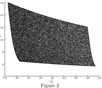
Achievable Set

In multicriterion optimization we consider various (competing) outputs of interest, say volume, V, and root temperature, s. Changing the dimensions of the fin by selecting differentαandβwill (say) decrease the volume of the fin, and hence material requirements - but also (typically) increase the fin base temperature. It is thus of interest to determine all possible operating points, that is, to generate the map of the “achievable set.” In general this will be prohibitively expensive unless one has recourse to a very low-dimensional representation such as the reduced-basis approximation.

We consider this problem for constant conductivities k_i = 1., i = 0, . . . ,4, and Biot number Bi= 0.001. We then select 100,000 points in the two dimensional design space [α, β] = [0.1,0.5]×[2.0,3.0] and evaluate our bounds forswith an error tolerance of 0.1%. Since in this design we wish to be sure that the actual temperature will be less than our prediction, we choose to construct our map based on s+_N. We are thus insured that at each design point the actual temperature will be lower than that on our curve.

4 6 8 10 12 14 16

19 20 21 22 23 24 25 26 27

s+_N

V

Figure 2

Acknowledgements

References

[ASB78]B. O. Almroth, P. Stern, and F. A. Brogan. Automatic choice of global shape functions in structural analysis. AIAA Journal, 16:525–528, May 1978.

[FR83]J. P. Fink and W. C. Rheinboldt. On the error behaviour of the reduced basis technique for nonlinear finite element approximations. Z. Angew. Math. Mech., 63(1):21–28, 1983.

[Kae00]R. Kaenel. Reduced basis methods and output bounds for partial differential equations. Master’s thesis, MIT, EPFL, 2000.

[MMO+00]L. Machiels, Y. Maday, I. B. Oliveira, A. T. Patera, and D. V. Rovas. Out-put bounds for reduced-basis approximations of symmetric positive definite eigen-value problems. C. R. Acad. Sci. Paris, S´erie I, 2000.

[MPR00]Y. Maday, A. T. Patera, and D. V. Rovas. A blackbox reduced-basis output bound method for noncoercive linear problems.College de France Series;also MIT-FML Report 00-2-1, 2000.

[Nag79]D. A. Nagy. Modal representation of geometrically nonlinear behaviour by the finite element method. Computers and Structures, 10:683–688, 1979.

[NP80]A. K. Noor and J. M. Peters. Reduced basis technique for nonlinear analysis of structures. AIAA Journal, 18(4):455–462, April 1980.