Seismic Response Reduction Of Structures Using Base Isolation

(1)

IJISET - International Journal of Innovative Science, Engineering & Technology, Vol. 2 Issue 2, February 2015. www.ijiset.com

ISSN 2348 – 7968

Seismic Response Reduction of Structures using Base Isolation

S.Keerthana1, K. Sathish Kumar2, K. Balamonica2

1_{Kongunadu College of engineering and technology, Thottiam, Trichy, India}

2_{CSIR-Structural Engineering Research Centre, Chennai,India}

[email protected]

Abstract:

Response of structuresand its components to earthquake vibrations is the major cause of damages and loss to lives. The intensity of loss of lives and damages can be reduced if the responses are controlled to a tolerable limit. The adverse effect of earthquakes led to the development earthquake protection devices. Among the three major types of protective systems namely passive, active and semi active, passive systems are simpler and easily adoptive.The base isolation system is one such passive control system that decouples the structure from the horizontal components of the ground motion by imposing flexible isolation elements with low horizontal stiffness between the superstructure and substructure. The isolation reduces the fundamental frequency of the structure that is much lower than the fixed base frequency and the predominant frequencies of the ground motion. In this paper the effect of base isolation on a structure has been studied by comparing the responses of the base isolated structure and fixed base structure. The influence of isolation characteristics on the seismic response of the structure has been investigated. The effect of using bilinear hysteretic isolation model on the response of the structure has been studied and compared with the linear models.

Keywords:Base isolation, decoupling, passive systems, response reduction

1. Introduction

Earthquakes are sudden violent movement of earth’s surface which releases quantum of energy. These energy travels in the form of seismic waves which affects the structures. According to the revised provisions of IS 1893 (Part 1): 2002 Code [1], the seismic zones of India have become more vulnerable and hence categorized to four zones. So it is important to design the structures with seismic resistance. The conventional seismic design mainly includes the lateral force resisting systems which concentrate on the formation of the plastic hinges. The main types of earthquake protective systems include passive, active and semi-active systems. In passive control [2] systems the devices do not require additional energy source to operate and are activated by the earthquake input. Active control systems

require additional power source, which has to remain operational during an earthquake and a controller to determine the actuator output. Hybrid control systems combine features of both passive and active control systems [3]. Since a portion of the control objective is accomplished by the passive system, less active control effort, implying less power resource, is required in the hybrid control system.

Recently additional supplementary devices are used for the control of the seismic vibrations. According to Kaplan[4]base isolation is one of the passive protective systems. The flexibility and the energy dissipation are the main characteristics of the base isolation system. The increase in period of the structure is mainly due to the flexible nature of the system and the energy dissipation is useful in limiting the displacement response of the structure [5].

2. Base isolation

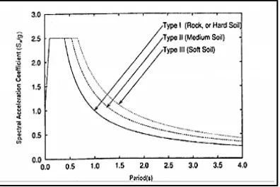
The concept of isolation is developed after the invention of the multilayer rubber bearings using the natural rubber or neoprene. The bearings are used in many bridge structures but their usage in the multistory buildings for vibration control is developing. The isolators are strong enough to carry the vertical loads of the structure as many thin steel shims are introduced between and laminated along with the rubber. In the lateral direction they are very flexible for shifting the natural period and avoiding the resonance of the structure. The typical response spectra of IS 1893- Part II is shown in the Fig. 1.

(2)

ISSN 2348 – 7968

Fig. 1: Response spectrum Curve

3. Case study

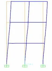
A three-storied building is modeled in the SAP 2000 software. An open frame building model with 2 bays in each X and Y directions with bay width as 1.5m and the height of each storey as 1.8m is modeled. The material properties of the frame elements and the area element are defined and M30 concrete grade is used. The rebar material properties are also given. The beams and columns of dimensions 150X200 mm are taken as frame elements. The slab in the building is assigned as a shell element with a thickness of 100mm. The rigidity of the beam column joints are given by rigid end offsets. No additional live loads are given to the model. The support condition at the bottom is made as fixed.

Then the free vibration analysis and time history analysis is done for the model to identify the natural modes and frequencies and the behavior under earthquake ground motion respectively. The fixed base model of the building done in SAP2000 is shown in the Fig.2.

Fig. 2:Building model used for analysis

4. Design of rubber isolator

The following expressions are used in the design of the rubber isolator [7].

(1)

(2)

(3)

(4)

Where, d=displacement of the rubber T= period of isolator

a= spectral acceleration

z = zone factor

K= Stiffness of the isolator m= mass of the structure t= thickness of the rubber layer

γ= shear strain

A= area of the isolator G= shear modulus

= Frequency of isolator

(3)

ISSN 2348 – 7968

5. Linear analysis

Free vibration and the time history analysis of the structure was performed for the case study considered. The behavior of the building modelin the presence of isolator and their performance during the strong ground motion given by the El Centro earthquake data are analyzed in the software.

During the free vibration analysis the natural period of the building model with fixed base conditions and isolated conditions are identified. It is found that there is a good increase in the period of the structure after installing the rubber isolator as link/support.The first mode shape of the structurewith and without the isolator is shown in the Fig 3 and Fig 4.

Fig. 3. Modal shape of the fixed base building model (0.19691 s) Fig. 4. Modal shape of the building with isolated base (2.55173)

Table 1: Time period variation between fixed and isolated base

Mode number Fixed base period(s) Isolated base _period(s)

1 0.235 2.554

2 0.196 2.551

3 0.181 2.487

4 0.078 0.231

5 0.063 0.225

6 0.060 0.125

7 0.050 0.088

8 0.038 0.061

9 0.038 0.056

6. Time history analysis

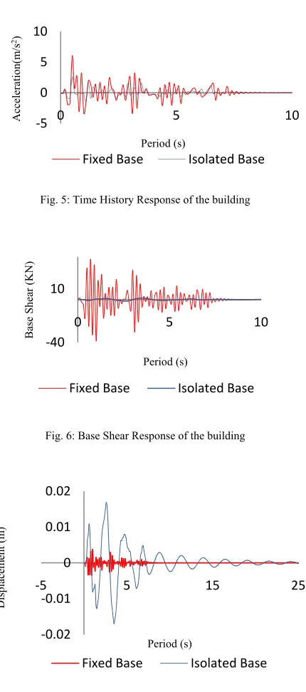
To understand the behavior of the structure for earthquakes, time history analysis using El Centro earthquake data is carried out. The reduction of response of the building model with and without the

isolator is shown in of Tables 2 and Fig 5-7.Reduction in the acceleration, base shear and increase in the displacement of the building model is observed.The increased time period of the structure tends to reduce the acceleration but it considerably increases the displacement.

Table 2: Comparison of response of fixed and base isolated structure

Response of the structure Fixed _Base

Rubber isolated

Base Reduction

Acceleratio n in X direction

(m/s2) at the top

Maximu

m 6.04 2.59 57%

Minimu

m -3.28 -1.38 58%

Displaceme nt in X direction (m) at the

top

Maximu

m 0.0062 0.0169 -63%

Minimu m

-0.0025 -0.0170 -85%

Base Shear in X direction

Maximu

m 37.72 12.06 68%

Minimu

(4)

Fig. 5: Time History Response of the building

Fig. 6: Base Shear Response of the building

Fig.7: Time History Displacement response at the top floor of the building

7.

Non-linear modelling of base isolation

The laminated rubber bearing used as an isolator exhibits hysteresisbehavior when loaded with cyclic loading. The typical hysteresis loop of a laminated rubber bearing can be modelled as bilinear i.e., the nonlinearity in the bearing is assumed to be bilinear as shown in the Fig 8. The parameters d1, F1, d2, and F2 are defined in the bilinear curve as the yield displacement, yield force, ultimate displacement and ultimate force respectively [9].

The hysteretic behaviour of a laminated rubber bearing can also be modelled linear, by using the effective stiffness Ke and the equivalent viscous damping coefficient ζe that depends on the ultimate displacement d2 and on the corresponding force F2 of the bilinear system. The linearization of the bilinear model can be made by using the Pre-yield stiffness (K), Post-yield stiffness (Ke) and the Ratio of pre-yield and post-yield stiffness (α). The effective stiffness from the bilinear model is calculated as equation 5

K

(5)

Fig. 8: Bilinear hysteresis loop model

The main parameter for the bilinear model is the effective stiffness i.e., the post yield stiffness value of the isolator and the additional damping value given by the hysteresis loop model. The formulation for the values of the effective stiffness and the additional damping is given below in equation 6.

F F αK d d

(6)

Kd αK d d

Kd 1 α μ 1 (7)

By simplifying and solving further,

K 1 α μ 1 (8)

Finally,K K α (9)

Additional damping provided by the hysteresis area,

ζe (10)

‐5 0 5 10

0 5 10

Acceleration(m

/s

2)

Period (s)

Fixed Base Isolated Base

‐40 10

0 5 10

Base Shear (KN)

Period (s)

Fixed Base Isolated Base

‐0.02 ‐0.01 0 0.01 0.02

‐5 5 15 25

Displacem

ent (m

)

Period (s)

(5)

(11)

The additional damping in terms of the effective stiffness is,

ζe (12)

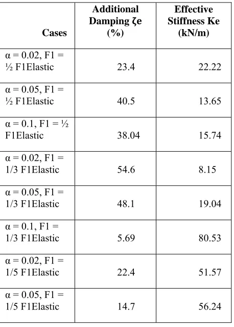
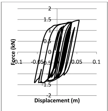
The additional damping incorporated in the system and the effective stiffness of the system can be determined from the equations 9 and 12. The post yield stiffness ratios (α) are assumed as 0.02, 0.05 and 0.1 for the laminated rubber isolator. The yield strength was assumed in a manner that the isolator will yield in half the value of force compared to the linear isolator. In this modus, the values of force are reduced at one-third, one-fifth and one-tenth of the linear yield force value so that the isolator will yield at that point and then the nonlinearity comes into report. Hysteresis loops were plotted for various cases from the results of various analyses that have been carried out (Fig9). Table 3 shows the additional damping and effective stiffness that is obtained for various cases.

Table 3: Computation of Additional damping and Effective stiffness

Cases

Additional Damping

(%)

Effective Stiffness Ke

(kN/m)

α = 0.02, F1 =

½ F1Elastic 23.4 22.22

α = 0.05, F1 =

½ F1Elastic 40.5 13.65

α = 0.1, F1 = ½

F1Elastic 38.04 15.74

α = 0.02, F1 =

1/3 F1Elastic 54.6 8.15

α = 0.05, F1 =

1/3 F1Elastic 48.1 19.04

α = 0.1, F1 =

1/3 F1Elastic 5.69 80.53

α = 0.02, F1 =

1/5 F1Elastic 22.4 51.57

α = 0.05, F1 =

1/5 F1Elastic 14.7 56.24

α = 0.1, F1 =

1/5 F1Elastic 24.2 31.76

α = 0.02, F1 =

1/10 F1Elastic 32.1 31.14

α = 0.05, F1 =

1/10 F1Elastic 10.5 17.41

α = 0.1, F1 =

1/10 F1Elastic 41.4 52.85

Fig.9.a: For the value α = 0.1, F1 = ½ F1Elastic

Fig.9.c: For the value α = 0.02, F1 = ½ F1Elastic

‐4 ‐3 ‐2 ‐1 0 1 2 3 4

‐0.1 ‐0.05 0 0.05 0.1

Fo

rc

e

(k

N

)

Displacemen

t (m)

‐4 ‐3 ‐2 ‐1 0 1 2 3 4

‐0.1

_Fo

rc

‐0.05 0 0.05 0.1

e

(kN

)

(6)

Fig.9.e: For the value α = 0.05, F1 = ½ F1Elastic

Fig.9.b: For the value α = 0.1, F1 = 1/3F1Elastic

Fig.9.d: For the value α = 0.02, F1 = 1/3 F1Elastic

Fig.9.f: For the value α = 0.05, F1 = 1/3 F1Elastic

Fig.9.g: For the value α = 0.1, F1 = 1/5 F1Elastic

Fig.9.i: For the value α = 0.02, F1 = 1/5 F1Elastic

‐4 ‐3 ‐2 ‐1 0 1 2 3 4

‐0.1_Force ‐0.05 0 0.05 0.1

(kN)

Displacement (m)

‐3 ‐2 ‐1 0 1 2 3

‐0.1_Force ‐0.05 0 0.05 0.1

(kN)

‐3 ‐2 ‐1 0 1 2 3

‐0.1_Force ‐0.05 0 0.05 0.1

(kN)

‐2.5 ‐2 ‐1.5 ‐1 ‐0.5 0 0.5 1 1.5 2 2.5

‐0.1_Force ‐0.05 0 0.05 0.1

(kN)

‐2 ‐1.5 ‐1 ‐0.5 0 0.5 1 1.5 2

‐0.1_Force ‐0.05 0 0.05 0.1

(kN)

‐1.5 ‐1 ‐0.5 0 0.5 1 1.5

‐0.1_Force ‐0.05 0 0.05 0.1

(kN)

(7)

Fig.9.k: For the value α = 0.05, F1 = 1/5F1Elastic

Fig.9.h: For the value α = 0.1, F1 = 1/10 F1Elastic

Fig.9.j: For the value α = 0.02, F1 = 1/10 F1Elastic

Fig.9.l: For the value α = 0.05, F1 = 1/10F1Elastic

The displacement of the structure is greatly reduced by considering the non-linear properties of the isolator. The nonlinear analysis reduces the displacement of the structure to the maximum of 37.79% while taking the post yield stiffness ratio (α) as 0.05 and the yield strength is taken as one tenth value of the elastic force.

Table 4: Displacement Reduction between linear and nonlinear analysis

Linear Analysis Displacement: 0.067m

Cases nonlinear analysis Displacement in (m)

Reduction %

α = 0.02, F1 =

½ F1Elastic 0.05629 18.77

α = 0.05, F1 =

½ F1Elastic 0.05585 19.41

α = 0.1, F1 = ½

F1Elastic 0.05499 20.65

α = 0.02, F1 =

1/3 F1Elastic 0.06005 13.34

α = 0.05, F1 =

1/3 F1Elastic 0.05895 14.94

α = 0.1, F1 =

1/3 F1Elastic 0.05692 17.86

α = 0.02, F1 =

1/5 F1Elastic 0.05719 17.47

‐2 ‐1.5 ‐1 ‐0.5 0 0.5 1 1.5 2

‐0.1_Force ‐0.05 0 0.05 0.1

(kN)

‐1.5 ‐1 ‐0.5 0 0.5 1 1.5

‐0.1_Force ‐0.05 0 0.05 0.1

(kN)

‐1 ‐0.8 ‐0.6 ‐0.4 ‐0.2 0 0.2 0.4 0.6 0.8

‐0.1 ‐0.05 0 0.05 0.1

Force

(kN)

‐1 ‐0.5 0 0.5 1

‐0.1_Force ‐0.05 0 0.05 0.1

(kN)

(8)

α = 0.05, F1 =

1/5 F1Elastic 0.05594 19.28

α = 0.1, F1 =

1/5 F1Elastic 0.05348 22.83

α = 0.02, F1 =

1/10 F1Elastic 0.04631 33.17

α = 0.05, F1 =

1/10 F1Elastic 0.04311 37.79

α = 0.1, F1 =

1/10 F1Elastic 0.04651 32.89

8.

Conclusions

Base isolation is one of the reliable techniques for earthquake resistant design of structures. The acceleration time history of the structure gets controlled if base isolation is used but it increases the displacement of the structure. The large displacements observed in the isolated structure can be controlledby designing the isolator in the nonlinear form which can be adopted easily. 58% reduction in the acceleration and 85% increase in displacement were observed. Further 38% reduction in displacement could be observed when the non-linear properties of the isolators were considered.

9. Acknowledgements

The paper is presented with the kind permission and approval of The Director, CSIR-SERC, Chennai, India.

References

[1] IS - 1893 (Part1), Indian standard criteria for

earthquake resistant design of structures, 2002.

[2] Buckle, I.G, Passive Control of Structures for Seismic

loads,Doctoral Thesis University of Nevada-Reno, United States of America, 2000

[3] Thakare P.P and Jaiswal O.R, Comparative Study of

Fixed Base and Base Isolated Building using Seismic

Analysis ,International Journal of Earth Sciences and

Engineering, Vol 4, pp. 520-525, October 2011

[4] Kaplan. K, Seismic Base Isolation and Energy

Absorbing Devices , European Scientific Journal, Vol

9, No-18

[5] Deb S.J, Seismic base isolation – An overview,

Current Science, Vol. 87, No. 10, November 2004

[6] Chandak N. R., Effect of Base Isolation on the

Response of Reinforced Concrete Building, Journal of

Civil Engineering Research, pp. 135-142, 2013

[7] Kelly.J.M., and Naeim.F, Design of seismic isolated

structures: From theory to practice, Nueva York, John

Wiley & Sons (1999)

[8] Uniform Building Code UBC (1997), Chapter 16,

Division IV—Earthquake regulations for Seismic-Isolated Structures

[9] Andriono, Takim, and Athol J. Carr. A simplified

earthquake resistant design method for base-isolated

multistorey structures.Bull NZ NatlSocEarthqEng 24.3