QC-MDPC: A Timing Attack and a CCA2 KEM
Edward Eaton1, Matthieu Lequesne23, Alex Parent1, and Nicolas Sendrier3??
1
ISARA Corporation, Waterloo, Canada {ted.eaton,alex.parent}@isara.com
2
Sorbonne Universit´es, UPMC Univ Paris 06, France 3
Inria, Paris, France
{matthieu.lequesne,nicolas.sendrier}@inria.fr
Abstract. In 2013, Misoczki, Tillich, Sendrier and Barreto proposed a variant of the McEliece cryptosystem based on quasi-cyclic moderate-density parity-check (QC-MDPC) codes. This proposal uses an iterative bit-flipping algorithm in its decryption procedure. Such algorithms fail with a small probability.
At Asiacrypt 2016, Guo, Johansson and Stankovski (GJS) exploited these failures to perform a key recovery attack. They introduced the notion of thedistance spectrum of a sparse vector and showed that the knowledge of the spectrum is enough to find the vector. By observing many failing plaintexts they recovered the distance spectrum of the QC-MDPC secret key.
In this work, we explore the underlying causes of this attack, ways in which it can be improved, and how it can be mitigated.
We prove that correlations between the spectrum of the key and the spectrum of the error induce a bias on the distribution of the syndrome weight. Hence, the syndrome weight is the fundamental quantity from which secret information leaks. Assuming a side-channel allows the ob-servation of the syndrome weight, we are able to perform a key-recovery attack, which has the advantage of exploiting all known plaintexts, not only those leading to a decryption failure. Based on this study, we derive a timing attack. It performs well on most decoding algorithms, even on the recent variants where the decryption failure rate is low, a case which is more challenging to the GJS attack. To our knowledge, this is the first timing attack on a QC-MDPC scheme.
Finally, we show how to construct a new KEM, called ParQ that can reduce the decryption failure rate to a level negligible in the security parameter, without altering the QC-MDPC parameters. This is done through repeated encryption. We formally prove the IND-CCA2 security of ParQ, in a model that considers decoding failures. This KEM offers smaller key sizes and is suitable for purposes where the public key is used statically.
Keywords: post-quantum cryptography, code-based cryptography, QC-MDPC codes, side-channel attack, timing attack, CCA2 security, key encapsulation
??
1
Introduction
Code-based cryptography is almost as mature as public-key cryptography it-self, dating back to 1978 with the invention of the original McEliece public-key encryption scheme [28]. This scheme, when used with (as originally proposed) binary Goppa codes, has largely resisted all cryptanalytic efforts, from both classical and quantum adversaries. Because of this, code-based cryptography is a strong candidate for post-quantum standardisation, with several variants [31,30] attempting to make improvements or refinements on the original design. Following [18,4], a new variant was proposed in 2013 using quasi-cyclic (QC) moderate density parity-check (MDPC) codes [29]. QC-MDPC codes use much shorter keys (about 10 kbits). This choice appears promising and the QC-MDPC scheme was recommended for further study by the report “Initial Recommen-dation of long-term secure post-quantum systems” of the European project PQCRYPTO [3]. Some hardware implementations of this scheme were published in [22] and [27].
The decryption algorithm of the QC-MDPC scheme is a variant of Gallager’s bit-flipping algorithm [19]. It is an iterative algorithm with a simple structure, very easy to implement, even on constrained devices. It has an inconvenient though, it is subject to failure with non-negligible probability. The algorithm proposed in the original paper [29] has adecoding failure rate (DFR) of 10−7.
While decoding errors may not represent a serious reliability issue, in a recent paper by Guo, Johansson and Stankovski (GJS) [20], the authors showed that these decoding failures actually do represent a very serious security issue. The authors exploited this DFR and managed to successfully recover the key by analyzing the error patterns that made the decryption fail. They found that these error patterns are correlated with the key. They introduce a new tool, the distance spectrum, to describe the correlation. They successfully use this correlation to perform their attack and give some hints on the reason why error patterns correlated in such a way are more prone to cause decryption failure.
The original QC-MDPC primitive is extremely vulnerable because the ad-versary may choose the error and even force a higher weight, in this case the attack of [20] recovers the key within minutes, when attacking a parameter set intended for the 80-bit classical security level. With a semantically secure con-version (CCA security, as in [23]) it requires 239.7 operations.
1.1 Our Contributions
with the Chernoff bound applied to the above mentioned bias. This opens the way to theoretical estimates for the cost of attacks related to the secret key distance spectrum recovery.
Next, by remarking that the syndrome weight is correlated to the decoding time, we perform a GJS type of attack by counting the number of iterations. This provides a timing attack which is very generic and can be applied to any variant of the bit flipping algorithm which is not protected against timing at-tacks. Moreover, it works regardless of the failure rate. To our knowledge, this is the first timing attack on this kind of scheme. This confirms a conjecture made by Maurich and G¨uneysu [25] that the number of iterations in the decoding procedure leaks secret information.
In Section 4 we demonstrate the power of this attack by showing experimental results of the timing attack on various parameter sets and decoding procedures. This shows that the attack is practical even against the 256-bit classical param-eter set. Additionally, we analyze and discuss how some other variations in the decoding procedure proposed in [27] affect the attack and its effectiveness.
Finally in Section 5, we show a new construction for a QC-MDPC-based KEM, called ParQ. This KEM uses QC-MDPC encryption as the underlying primitive, and does not need to alter the parameter set of the primitive itself. The scheme works by creating multiple independent encapsulations of the same key, so that a decapsulation failure only occurs if a decoding failure happens for each ciphertext. This causes the decapsulation algorithm to only fail with negligible probability, and so it entirely eliminates the possibility of using decoding failures to recover the key with the GJS attack. This scheme does not increase key sizes at all, and only increases the size of the encapsulation by a small factor (3 – 12×). We provide a comprehensive proof of IND-CCA2 security of the scheme, and analyse the KEM compared with other code-based key transport methods. Our proof considers the possibility of decoding failures. Other CCA2 constructions [23,26] did not consider this, which is why the GJS attack was able to break CCA2 security. Most commentary on mitigating the GJS attack has focused on either altering the parameters of QC-MDPC to decrease the DFR or using the keys ephemerally. Through our scheme we show that there is a third option that can address decoding failures at the protocol level.
1.2 Related Work
The McEliece cryptosystem was originally proposed in [28], and low density parity-check codes were proposed in [19]. The QC-MDPC variant of McEliece was proposed in [29]. The key-recovery reaction attack we focus on in this paper was shown in [20]. In [17], the authors analyzed how the observations from [20] applied to the case of LDPC McEliece [30], showing that the attack also worked on soft decision decoding procedures.
Side-channel timing attacks [24] on McEliece systems other than QC-MDPC have been considered for example in [33,34,35] which has motivated the need for constant-time implementations [7,13]. In [25,11,12], the authors demonstrated several power-analysis side-channel attacks on QC-MDPC, and [25] conjectured that it might be possible that the number of decoding rounds leaks secret infor-mation. To our knowledge, our paper is the first to conclusively show that this is in fact the case.
CCA2 conversions for McEliece systems have been considered before, most notably in [23]. General conversions for designing CCA2 KEMs from OW-CPA systems were studied in [15]. Other key exchange and key encapsulation schemes related to QC-MDPC include [5,13,14,26].
A line of constructions beginning with [32], and applied to McEliece in sev-eral follow-up works [16,36] explored the concept of the k-repetition paradigm for encryption. This paradigm bears some resemblance to our parallel KEM in Section 5, although these constructions are different and have a different goal: CCA2 security without random oracles.
2
QC-MDPC McEliece and the GJS Attack
2.1 Quasicyclic Moderate Density Parity Check McEliece
QC-MDPC-McEliece is a public key encryption method consisting of three al-gorithms. It is defined by four parameters, n, k, w, and t. The key generation algorithm QCMDPC.KeyGen constructs an (n, k)-linear quasicyclic code, con-sisting of a generator matrix G (the public key) and a parity check matrix H (the secret key), for which each row has weight w. The encryption algorithm
QCMDPC.Enc encrypts a plaintext x ∈ IFk2 by calculating the corresponding codeword to x, xG and adding an error e of weight t to obtain the ciphertext c=e+xG. The decryption algorithmQCMDPC.Decdecodesc back toxGand recoversx.
While QC-MDPC can allow forkto be any divisor ofn, we will consider the case of n/k = 2. We letE denote the set of e ∈IFn2 with Hamming weight t. Note that the size of each block,r= (n−k) =k.
Algorithm 1 QCMDPC.KeyGen
Input: Security parameter 1λ. Output: Public keypk, secret keysk.
1: Generateh0, h1∈IFk2, both with weightw/2.
2: LetH= [H0|H1], whereH0 andH1 arek×kmatrices generated fromh0 andh1 by cyclically rotating them.
3: SetG= [Ik|Q], whereIkis thek×kidentity matrix,Q= (H1−1H0)T.
Algorithm 2 QCMDPC.Enc
Input: Public keypk=q, plaintextx∈IFk
2, error vectore∈E. Output: Ciphertextc∈IFn2.
1: ReconstructG= [Ik|Q] by cyclically rotatingqto obtainQ. 2: returnc=e+xG.
Algorithm 3 QCMDPC.Dec
Input: Secret keysk, public keypk, and ciphertextc∈IFn2. Output: Plaintextx∈IFk
2 and error vectore∈E, or decryption failure symbol⊥. 1: Reconstruct parity-check matrixH= [H0|H1], and generator matrixG= [Ik|Q]. 2: Run the decoding procedure oncwith parity-check matrixHto recover codeword
xG. If a decoding failure occurs, return⊥. 3: Recoverxfrom the firstkbits ofxG. 4: Recovere=c−xG.
5: return(x, e).
Multiple parameter sets for QC-MDPC have been proposed for multiple secu-rity levels. Our interest is in the 80-bit and 256-bit classical secusecu-rity sets (which corresponds to at least 40-bit and 128-bit quantum security) that were originally proposed in [29], and have been further discussed in [5].
Classical bit-strength n k w t
80 9602 4801 90 84
128 20 326 10 163 142 134
256 65 542 32 771 274 264
2.2 QC-MDPC Decoding Procedure
The original paper on MDPC codes [29] proposes to use a hard decision version of Gallager’s bit-flipping algorithm for decoding LDPC codes [19]. The main idea is the following. At each iteration, the algorithm computes the number of un-satisfied parity-check equations associated to each bit. Each bit that is involved in ≥b unsatisfied equations is flipped, for bsome threshold, and the syndrome is recomputed. This repeats until the syndrome becomes zero. In practice, the algorithm stops after fixed number of iterations and this is considered a decoding failure.
For our main analyses we use decoder D1 from [27] with fixed thresholds
{95,85,80,76,74,73,72,72}.D1is a modification of Gallager’s algorithm which updates the syndrome in place after each bit flipped. Algorithm 4 is the normal out-of-place bit flipping algorithm and Algorithm 5 is the in-place version.
Algorithm 4 Iterative bit flipping decoding algorithm
Input: c= (c0, . . . , cn−1)∈IFn2,H= (h(0), . . . , h(n−1))∈IFr
×n 2
s←H·c| .compute the syndrome
whiles6= 0do
fori= 0, . . . , n−1do
if hs, h(i)i ≥bthen .if number of unsatisfied equations≥thresholdb
ci←ci⊕1 .flip theith bit
s←H·c|
returnc
Algorithm 5 In-Place: Iterative bit flipping decoding algorithm
Input: c= (c0, . . . , cn−1)∈IFn2,H= (h(0), . . . , h(n−1))∈IFr2×n
s←H·c| .compute the syndrome
whiles6= 0do
fori= 0, . . . , n−1do
if hs, h(i)i ≥bthen .if number of unsatisfied equations≥thresholdb
ci←ci⊕1 .flip theith bit
s←s⊕h(i) returnc
approach gives the best results so far, both in terms of decryption failure rate and average number of iterations.
In both cases, until now the thresholds were claimed as experimental results with no explanation on the way they were generated. In appendix B we discuss a procedure to obtain such thresholds for any security parameters.
2.3 The GJS Attack
The key recovery attack in [20] is a reaction attack. It takes advantage of the decoding failures that occasionally occur during decryption. It assumes only that an adversary is able to tell when such an error has occurred, for example because a request for resend is sent back. It consists of two steps. The first step is to calculate thedistance spectrumof the secret key (or one part of the secret key), based on observing a large number of error vectors that resulted in a decoding failure. The second step is to reconstruct the secret key based on its distance spectrum.
In this paper, we will focus our attention on the first step. Reconstructing the secret key from the distance spectrum has been analysed before [20,17], and shown to be fairly fast and simple as compared to the first step, and is an entirely offline computation, requiring no communication.
Definition 1 (Distance Spectrum). The distance spectrum of a vector h∈
bits of hat distanceδ. The distance are counted cyclically.
∆(h) =
δ: 1≤δ≤jr
2
k
,∃(i, j),
0≤i < j < r, h[i] =h[j] = 1,
min{j−i, r−(j−i)}=δ
whereh[i] denotes theith entry of the binary vectorh.
1
1 1 1
0 0
0
0 0
1
1 2 3
4 4
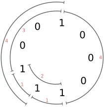
Fig. 1: Distance spectrum of 1001000112
For example, the distance spectrum of the vector 1001000112 is {1,2,3,4} (fig. 1). Note that any cyclic shift or reversal of a vector will result in the same distance spectrum. In [20,17], it was shown how to quickly reconstruct a vector (up to a reversal or cyclic shift) from a distance spectrum. The first step of the GJS attack is to find the distance spectrum of the first halfh0of the secret key (h0, h1). From this,h0can be computed, which allows us to also calculateh1by elementary linear algebra.
In order to analyse more precisely the results, we need to take into account the fact that some distances may appear more than once.
Definition 2 (Distance Spectrum with multiplicity). The distance spec-trum with multiplicity of a vector h∈IFr2, denoted ∆µ(h), is a vector ofINb
r 2c
such that for every distance 1 ≤ δ ≤ r 2
, its δth component ∆µ(h)[δ] is the number of existing sets of two non-zero bits ofhat distanceδ. The distance are counted cyclically.
Example 1. Forh= 00110000112(see Figure 1), then∆µ(h) = [2,1,1,2]. In general we can see that if a vector h0 ∈ IFk2 has weight w0, then the distance spectrum with multiplicity ofh0will be a vector of sizebk/2csuch that the sum of the entries of∆µ(h0) is w20
.
Observation 1 (GJS, Key Observation).When a distance in the error vec-tor used in a QC-MDPC encryption matches a distance in the distance spectrum of the secret key, a decoding failure is less likely to occur.
Based on this observation, it was noticed that by carefully calculating the decoding failure rate for errors that have a given distance vs. those that do not, the multiplicity of that distance in the secret key’s distance spectrum can be correctly guessed. Note that this observation applies to each half of the error vector (and parity check matrix) independently. So when we refer to the distance spectrum of the error or parity-check matrix, we mean the distance spectrum of the firstkbits, unless stated otherwise.
Algorithm 6 was proposed in [20] for attacking the CCA security of a QC-MDPC implementation.
Algorithm 6 GJS CCA attack
1: Initializeobservedd= 0 andf ailedd= 0 ford∈ {1, . . . ,bk/2c}. 2: fori= 1 toM do
3: Sendc=QCMDPC.Enc(x, e) with a uniformly randome= [e0||e1] to target. 4: ford∈∆(e0)do
5: Incrementobserveddby 1. 6: if Decoding failed forcthen 7: Incrementf aileddby 1.
8: returnf ailedd/observeddford∈ {1, . . . ,bk/2c}.
The resulting values, f ailedd/observedd for each dgive an estimate of the decoding failure rate for error vectors withdin their distance spectrum. We can then recover the distance spectrum, identifying the multiplicity of each distance from the following observation:
Observation 2 (GJS).For a fixed key, the decoding failure rate for error vec-tors withdin their distance spectrum is inversely proportional to the multiplicity ofdin the distance spectrum of the key.
For large enough values ofM, the decoding failure rate clearly separates into bands. These bands exactly correspond to the multiplicity of that distance in ∆(h0). This allows an attacker to recover∆(h0), and thus the secret key.
3
Analysis and Timing Attack
3.1 Correlation
Our attack is based on the fact that the average syndrome weight is slightly different if the relative position of non-zero bits in the key and the error are correlated.
For the sake of simplicity, in this section, we will consider a parity-check matrix made of one single circulant block in H ∈IFk2×k instead of two. We will see later that the practical results are the same. We denote byh∈IFk2 the first row of the matrixH. The variabletstill represents the weight of the errore, so here the numerical value oft should be half its usual value.
Without any information. Let us suppose that we do not have any informa-tion on the key. For a random key vectorhof sizekand weightdand a random error vectoreof sizek and weightt, denote byf(k, d, t, b) the probability that the scalar product in IF2is of parityb:
f(k, d, t, b) := Pr[hh, ei=b] =
d
X
i=0, iis of parityb d i
k−d
t−i
k t
.
The average syndrome weight of an erroreand a parity-check matrix gener-ated by cyclic shifts ofhisktimes the probability that a bit is non-zero (see [9, page 91]), that is:
E[wt(H·e|) ] =k·f(k, d, t,1).
Case of two consecutive non-zero bits in the key. Now, suppose the key vectorhhas` times two consecutive non-zero bits. Let us observe the shifts of the vector:
shift(h) = 1 1 u,wt(u) =d−2 ` times
shift(h) = 1 0 u,wt(u) =d−1 d−`times
shift(h) = 0 1 u,wt(u) =d−1 d−`times
shift(h) = 0 0 u,wt(u) =d k−2d+`times.
Suppose that the first two bits of the error vector are non-zero, that is:
e= 1 1 u,wt(u) =t−2 .
E[wt(H·e|) ] = ` f(k−2, d−2, t−2,1)
+ 2(d−`) f(k−2, d−1, t−2,0) + (k−2d+`)f(k−2, d, t−2,1).
(1)
Contrary to the previous result, this is an approximation. Indeed, this model assumes that the rest of the vector (denoted by u) is random for each shift. It does not take into account the covariance between the bits of the syndrome. Previously we were averaging on all the lines and the covariance was therefore null, while here the fact that we group the rows depending on the value of the first two bits breaks the symmetry. Still, we will see that the approximation is close to the real value and we can neglect the correction term for the rest of the study.
Exploiting the leak. Suppose that we only consider error patterns start-ing with two consecutive non-zero bits, the syndrome weight is expected to be slightly different on average, depending on ` the number of times two consecu-tive bits are non-zero in the key vectorh. Moreover, the expected value varies linearly with`. Therefore, if we observe enough values of the syndrome weight, we can recover the value of`.
Definition 3 (Average syndrome weight with multiplicity). Let us de-note by D` the following set:
D`:=
n
(h, e)∈IFk2×IFk2|wt(h) =d,wt(e) =t, δ∈∆(e), ∆µ(h)[δ] =`o.
The average syndrome weight with multiplicity σ¯` is the expectation of the syndrome weight for a uniform distribution of (h, e)overD`:
¯
σ`:=E(h,e)∼U(D`)[wt(H·e
|) ].
From the equation (1) in Section 3.1 we know that we can approximate ¯σ` by:
¯
σ`= ` f(k−2, d−2, t−2,1) + 2(d−`) f(k−2, d−1, t−2,0) + (k−2d+`)f(k−2, d, t−2,1).
withf(k, d, t, b) :=
d
X
i=0, iis of parityb d i
k−d
t−i
k t
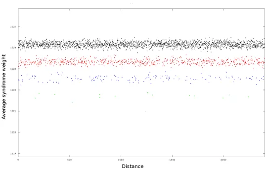
Comparison with measured values. The values of ¯σ` correspond to the different clusters that we can see on the figures. According to the approximation, the value of ¯σ`is linear in the multiplicity: ¯σ0−σ¯`=`·(¯σ0−σ¯1). This is consistent with what we observe..
Fig. 2: Attack on the syndrome weight (1 block): Average syndrome weight per distance, 105 samples. The color of the distances indicate their multiplicity in the key spectrum (black = 0, red = 1, blue = 2, green = 3)
When comparing the values to those measured on Fig. 2, we can see that the measured ¯σ0is slightly lower than the approximated value, and on the contrary ¯
σ1 is slightly higher. This error is due to the approximation that neglects the covariance. When performing the same experiment on parameters for LDPC codes, where the covariance is much smaller, the measures correspond exactly to the computed values.
As a consequence, the real distance ¯σ0−¯σ1is smaller than the one computed using equation (1). Hence, the theoretical analysis gives an interesting bound on the relative distanceε= σ¯0−σ¯1
k :εmeasured< εcomputed.
Hypothesis testing. Each syndrome is the result ofkscalar products between the error and a parity-check equation. When the error contains a distance present in the spectrum of the key with multiplicity `, the average syndrome weight is ¯
σ`, this means that on average ¯σ`of thekparity-check equations are not verified. Hence, under the independence assumption, we can see each bit of the syndrome as a Bernoulli trial satisfied with probability ¯σ`
k .
Here, our goal is to decide for each distance δ whether or not δ is in the distance spectrum of h. We do not care about the multiplicity. Formally, we want to distinguishD0 from ∪`≥1D`. Let us byD≥1:=∪`≥1D`. We can define ¯
σ≥1 on D≥1 just like we defined ¯σ` on D`. The sets are disjoint so we have ¯
σ≥1=
P
`≥1σ¯`|D`| P
`≥1|D`| .
from a random binary variable with success probability p1 := ¯σ≥1. This is a classic problem of hypothesis testing.
Note that for our parameters, the size ofD` for`≥2 is negligible compared toD1, hence there is no practical need to distinguish ¯σ1 from ¯σ≥1.
Sample size. There is a lot of literature about hypothesis testing, and in par-ticular a theorem from Chernoff [21] concerning such cases.
Proposition 1 (Chernoff ’s bound).Let0< p <1, letX1, X2, . . . , XN be in-dependent binary random variables, withPr[Xk= 1] =pand letSN =
PN k=1Xk
N .
Then for any t≥0,
Pr[|SN −p| ≥t]≤2e−2N t
2
.
This can be used to understand how the number of samples required to find the key evolves. Here we want to distinguishp0fromp1, we will use p0+p2 1 as the decision threshold. Chernoff’s bound states that we should haveN∼ 1
ε2 repeated
Bernoulli trials for the decision test to be relevant, whereε=|p1−p0|=σ¯0−kσ¯1 is the distance between the two outcomes.
To decide whether a particular distanceδis in the spectrum or not, we need to compute the mean ofN Bernoulli trials, but each syndrome weight is already the sum of the results ofkBernoulli tests. Hence, we need to observe the weight of Nk syndromes. These syndromes need to be in one of theD`, this means that the distanceδ needs to be in the spectrum of the error pattern that generates the syndrome. As the error patterns are generated uniformly, we proceed by rejection sampling to ensure this condition. The number of vectors of sizekand weightwthat do not contain a particular distance isQw−1
j=0(k−3j), so neglecting the cases of multiplicity we obtain a good approximation of the frequency of such vectors with:
α:= Pr(δ∈∆(e))≈1−
Qb
t 2c−1
j=0 (k−3j)
Qbt
2c−1
j=0 (k−j) .
Hence, to decide whether or notδ∈∆(h), we need to observe the decoding of N
α·k syndromes, withN ∼ 1
ε2. As we use the same data to decide for all distances,
this is the number of samples needed to recover the whole spectrum.
3.2 Attack on the Syndrome Weight
Attack Model. The scenario for our attack is the following. Eve can encrypt random messages using the QC-MDPC scheme described in 2.1 and Alice’s public key. She has access to the plaintext but cannot choose the messages. She sends the messages for decryption. Whenever the device decodes a message sent by Eve, she has a way to observe the weight of the syndrome.
a particular implementation and on the abilities of the attacker. The point is to establish through a simulation that some secret information leaks from the syndrome weight and to compare the cost of that simulation with the theoretical analysis of the previous section.
Eve Alice’s Decoder
m←IFk2
e←−$ IFn2,wt(e) =t c=GAlice·m |+e
Decode(c, HAlice) :
s←HAlice·c|
σ σ←wt(s)
. . .
We suppose that Eve’s error patterns are randomly generated. Indeed, in the scheme, semantically secure conversions ensure that the error patterns are random [23]. If we allow Eve to choose the error patterns, this will only make the attack easier, as in [20].
Contrary to [20], we collect information from all the error patters, not only those leading to a decoding failure.
Attack on Syndrome Weight. Our goal is to compute the distance spectrum of Alice’s private key. For each distanceδbetween 1 andbk
2cwe want to decide whether or notδ∈∆(hAlice). As we have seen in 3.1, for each distanceδ∈∆(e), the expected average weight of the syndromeσ=wt(s), wheres=HAlice·c|= HAlice·e|, is expected to be different ifδ∈∆(hAlice).
Hence, the idea is, for each distanceδ, to compute the average value of the syndrome weightσfor error patterns e such thatδ∈∆(e). The error patterns are generated randomly and each errore can be used to obtain information on all the distances in its spectrum. This leads to algorithm 7.
Following the discussion in Section 3.1, we will takethreshold= ¯σ0+¯σ1
2 .
3.3 Attack on Iteration Count
Now that we know that the syndrome weight leaks information, any parameter correlated to this quantity could be used for a side channel attack. An interesting parameter that is often easy to measure is the number of iterations of a loop.
The decoding algorithm for QC-MDPC codes is an iterative algorithm with no termination proof. The number of rounds needed to correct the errors varies. This has been studied by in [10]. As mentioned in Section 2.2, the algorithm depends on the way we chose the thresholds. For most instances, using fixed or variable thresholds, the algorithm usually corrects the error in 3 rounds, but some instances need 4, 5 or even more iterations. Usual implementations abort after a certain number of rounds (around 10), this is what was used for the attack in [20].
Algorithm 7 Computing the distance spectrum
Input: N the size of the sample, oracle access to the decoder SyndromeCount←(0, . . . ,0)∈INbk2c
OccurenceCount←(0, . . . ,0)∈INbk2c ∆←(0, . . . ,0)
for0≤i≤N−1do
e←−$ IFn2,wt(e) =t
σ←OracleDecoder(e) . σ=wt(e·HAlice|)
forδ∈∆(e)do
SyndromeCount[δ] +=σ
OccurenceCount[δ] += 1 for1≤δ≤ bk
2cdo
if SyndromeCount[δ]/OccurenceCount[δ]<thresholdthen
∆[δ]←1 return∆
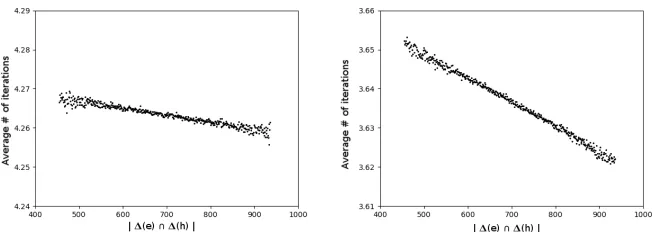
The more distances appear both in spectrum of the error and in the spectrum and the key, the fewer the number of iterations needed to decode on average. This appears clearly on Fig. 3. We note that the correlation is slightly more important on Fig. 3 when we use variable thresholds than with fixed theresholds (the average value is lower for variable thresholds, but the same scale is used for both figures).
Fig. 3: Average number of iterations needed for decryption, depending on the size of the intersection of the spectrum of the error and the spectrum of the key. 229samples, 128-bit security QC-MDPC scheme, decoding with fixed thresholds (left) and variable thresholds (right). Note that use of variable thresholds results in stronger correlation.
To obtain the spectrum, Eve uses the exact same data collection algorithm: for every distance in the spectrum, she computes the average number of iterations needed to correct an error containing this distance.
This works well and it is possible to fully recover the distance spectrum with variable thresholds using 225samples on 80-bit security QC-MDPC scheme, 225 samples for 128-bit security parameters (see Fig. 6) and 228 samples for 256-bit security parameters. For fixed thresholds, we manage to recover the spectrum for 256-bit security with 228 samples.
Algorithm 8 Timing attack on QC-MDPC
1: Initializeobservedd= 0 anditerationsd= 0 ford∈ {1, . . . ,bk/2c}. 2: fori= 1 toM do
3: e←−$ IFn
2,wt(e) =t 4: c←QCMDPC.Enc(x, e) 5: Sendcto target.
6: n←number of iterations (from side channel). 7: ford∈∆(e0)do
8: observedd+= 1.
9: iterationsd+=n.
10: Returniterationsd/observeddford∈ {1, . . . ,bk/2c}.
4
Experimental Results
Results of Syndrome attack. The spectrum recovery algorithm was first tried on a simplified version of the scheme using only one block, in order to compare to the expected behaviour. The result is striking. Using the usual parameters for 80-bit security, with one hundred thousand samples, the spectrum appears very clearly and we can even see the multiplicities, that is, distances that appear several times in the key, see Fig. 2. When pushing to one billion samples, there is no room for confusion.
When performing the same experiment on the real QC-MDPC scheme with two blocks, we obtain similar results. The attack is performed on each block separately, that is for each error pattern, we added the syndrome weight to the counters of all distances present in the first half of the error to recover the spectrum of the first block. Because there is no correlation between the two halves of the error pattern, the presence of the second block acts as a random noise added to the syndrome weight. Hence the only difference is that we need more samples to reduce the variance and distinguish well which distances are in the key spectrum. Note that it is possible to compute the spectrum of both blocks at the same time, so there is no need to double the number of samples to recover the second block.
samples, we can fully distinguish the spectrum. The same attack requires 223 samples for 128-bit security parameters and 225for 256-bit security parameters.
Fig. 4: Average syndrome weight per distance, (from left to right, from top to bottom) 214, 216, 218 and 220 samples, 80-bit security QC-MDPC scheme. The color of the distances indicate their multiplicity in the key spectrum (black = 0, red = 1, blue = 2, green = 3, purple≥4)
This attack was also performed when another error is added to the syndrome, like in the Ouroboros scheme [14] (with an additional error of weight 3d). Again, this only adds random noise and we can recover the spectrum with around a few million samples for the 80-bit security parameters.
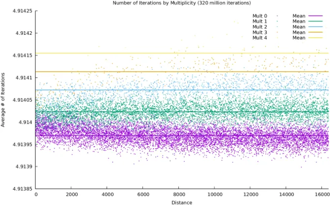
Results of iteration attack. After running algorithm 8 we collect data corre-sponding to the average number of iterations it took to decode an error whend is present. The resulting plots (fig. 5) look very similar to the plots of the decod-ing failure rate that result from Algorithm 6. Once the bands have completely separated, the distance spectrum (and thus the secret key) can be recovered in the same way it was in the GJS [20] attack.
Fig. 5: Attack using the number of decoding iterations against parameters for 256-bit security with fixed threshold decoding.
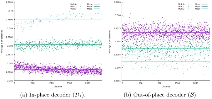
4.1 In-place decoder vs. out-of-place decoder
We observed that changes to the decoding algorithm can have a significant im-pact on the information gathered during the attack.
D1 uses in-place updates to the syndrome which seems to cause some asym-metry in the errors with respect to distance. For example, in Figure 5 the bands converge as distance increases.
Postponing the updates until the end of each iteration (usingB from [27]) seems to eliminate this asymmetry and reduces the correlation between number of iterations and distance multiplicity. This may reduce the efficiency of the attack.
Figure 7 shows a direct comparison between these two types of decoders. Note that the relationship between number of iterations and multiplicity is inverted between decoders.
We are not sure why this is the case but give a possible explanation for the behaviour. When distances match the resulting behaviour is a decrease in total changes to counters (both correct and incorrect). As noted in [20] this decreases the error rate since it decreases the probability of an incorrect change. It also decreases the expected number of bits flipped which could cause an increase in the expected number of iterations.
When multiple bits are flipped at once in the out-of-place decoder the benefit of a correct flip early in an iteration is removed so it is possible that benefit of early flipping is dominated by the increased chance of an incorrect flip.
2.786 2.7865 2.787 2.7875 2.788 2.7885 2.789 2.7895 2.79 2.7905
0 500 1000 1500 2000
A
verage # of Iterations
Distance Mult 0 Mult 1 Mult 2
Mean Mean Mean
(a) In-place decoder (D1).
3.3055 3.306 3.3065 3.307 3.3075 3.308 3.3085
0 500 1000 1500 2000
A
verage # of Iterations
Distance Mult 0 Mult 1 Mult 2
Mean Mean Mean
(b) Out-of-place decoder (B).
5
Eliminating Decoding Failure Vulnerabilities
In this section we present ParQ — A KEM constructed from repeating a QC-MDPC encryption scheme in order to eliminate the effect of decoding failures. The general idea is for the ciphertext to include several independent encapsu-lations of the same key in such a way that the scheme achieves CCA2 security, and so that a decapsulation failure occurs in ParQ only if a decryption failure occurs in every instance of the underlying QC-MDPC scheme. As current esti-mates for the failure rate indicate that failures occur at a rate of roughly 2−23, this suggests that a small amount of parallelization (3 – 12×) will make decap-sulation failures occur in ParQ at a negligible rate, thus removing the possibility of implementing a reaction attack based on these failures.
5.1 ParQ — A Parallelized QC-MDPC KEM
ParQ is largely characterized by the same parameters as other QC-MDPC code-based schemes, specifically,k, the plaintext length,n= 2k,w, the weight of the secret key, andt, the weight of the error. In addition to these parameters, ParQ has the parameter P, denoting the degree of parallelization. P must be greater than or equal to 2, and should generally be chosen to be in the range of 3 – 12. ParQ is described by three algorithms:ParQ.KeyGenfor key generation (omitted since it is the same as algorithm 1),ParQ.Encfor encapsulation, and ParQ.Dec
for decapsulation. It uses three functions which we model as random oracles,
ErrGen,PRF, and KDF, which map ontoE, IFk2, and{0,1}
λ, respectively.
Algorithm 9 ParQ.Enc
Input: Public keypk, a seeds∈ {0,1}k .
Output: Session keyK, key encapsulationC= (c1, . . . , cP). 1: fori= 1 toP do
2: Letei=ErrGen(s||i). 3: Computexi=s⊕PRF(ei||i).
4: Computeci=QCMDPC.Enc(pk, xi, ei). 5: ComputeK=KDF(s).
6: Return session keyK, key encapsulationC= (c1, . . . , cP).
5.2 Overview of IND-CCA2 reduction for ParQ
Algorithm 10 ParQ.Dec
Input: Secret keysk, public keypk, and encapsulationC= (c1, c2, . . . , cP). Output: Session keyK, or decapsulation failure symbol⊥.
1: fori= 1 toP do
2: Run (xi, ei)←QCMDPC.Dec(sk, ci).
3: if QCMDPC.Decsuccesfully decoded for the first timethen 4: Set used indexj=i.
5: if QCMDPC.Decfailed to decode fori= 1 toP then 6: Return decapsulation failure⊥.
7: Computes=xj⊕PRF(ej||j).
8: ComputeK, C0= (c01, c02, . . . , c0P)←ParQ.Enc(pk, s). 9: if ci=c0ifor alli∈ {1, . . . , P}then
10: Return K. 11: else
12: Return decapsulation failure⊥.
Theorem 1. Let A be an adversary capable of winning the IND-CCA2 secu-rity game with the ParQ KEM with qd decapsulation queries and qErrGen,qPRF,
and qKDF queries to the random oracles ErrGen, PRF, and KDF respectively, in
time t and with advantage . Then there exists a reductionB that uses A as a subroutine by simulating the IND-CCA2 environment in order to break the OW-CPA security of QC-MDPC McEliece, in time ≈t and with success probability γ(/P −δ), where δ is negligible and γ is negligibly close to 1 in the security parameter.
In order to establish IND-CCA2 security via a reduction from OW-CPA, we need to establish how to embed the given OW challenge c∗ into an IND challenge (Section 5.4), and how to successfully respond to decapsulation queries (Section 5.5). Then we need to show that the simulation satisfies several key properties: that the simulated challenge is indistinguishable from a real challenge (Section 5.4), that an adversary’s ability to solve the IND challenge allows the simulation to solve the OW challenge (Section 5.4), and that the simulated responses to decapsulation queries are indistinguishable from actual responses to a decapsulation query (Section 5.5).
In ParQ, we have that ei = ErrGen(s||i) and xi = s⊕PRFi(ei), or s = xi⊕PRFi(ei). So for any possiblecandi, there is at most onesassociated with it such thatc=QCMDPC.Enc(s⊕PRF(ErrGen(s||i)||i),ErrGen(s||i)).
5.3 Simulating the Random Oracle
query is made, we first check if it has been queried before, and if so, respond with the same response made before. We then specify how to handle new queries.
For new queries to ErrGen of the form s||i we choose a uniformly random error vector e ∈ E. We then also calculate x = s⊕PRF(e||i) and add e and c=QCMDPC.Enc(x, e) to the table. We then respond with e.
For new queries to thePRForacle of the forme||iwe first check and see ifeis the error vector associated with the challenge ciphertextc∗. We do this by using the generator matrixGto see ifc∗−eis a codeword. If so, then we have solved the challenge. Otherwise, generate a uniformly random string from{0,1}k, add it to the table and respond.
New queries toKDFcan simply be handled by responding with a uniformly random{0,1}λ.
5.4 Challenge Injection
As we are attempting to solve an OW-CPA challenge, we are given a public key Gand a ciphertextc∗ and asked to find the (x∗, e∗) such thatc∗ =x∗G+e∗.
To simulate a challenge, we will first select a uniformly random indexj ←−$ {1, . . . , P}. Then, we will select a uniformly random seed s∈ {0,1}k. We will run the encapsulation algorithmParQ.Encon the seeds, except that we willnot queryErrGen(s||j) to generateej, and thus not generatexj andcj. Thus we will have c1, . . . , cj−1, cj+1, . . . , cP andK.
To finish the challenge encapsulation, we will select a uniformly random bit b ∈ {0,1}. If b = 0, we will send K, and if b = 1 we will send a uniformly random K0 ∈ {0,1}λ. We will send C = (c
1, . . . , cj−1, c∗, cj+1, . . . , cP) as the encapsulation.
OW Challenge Solution Extraction. We need to show that the adversary’s advantage in solving the IND-CCA2 challenge corresponds to an extractor’s abil-ity to solve the OW-CPA challenge. Note that the only way for an adversary to distinguish the correct key from an incorrect one is by querying thesassociated with each ci to the KDF oracle. Without having done this, the adversary has no information on K and so she has no advantage in distinguishing a proper K from a random one. Therefore, the adversary’s advantage in distinguishing corresponds exactly to their ability to query (and thus find)s.
First, we show that the adversary’s probability of queryingstoKDFwithout having queried anei for one of theci’s toPRF(along withi) is negligibly small. Without having queried someei toPRF, the plaintext valuesx1, . . . , xp pro-vide no information ons. Recall thats=xi⊕PRF(ei||i). Then (x1, . . . , xP) can be thought of as P maskings of the same value s, with independent masking values. This contains no information about s, unless the adversary has queried at least oneei toPRF.
to PRF, then both (x1, . . . , xP) and (e1, . . . , eP) give no information about s, and so the encapsulationC= (c1, . . . , cP) does not.
So we have shown that unless the adversary queriesei||i to PRF or s||i to
ErrGen (for any i), the encapsulationC = (c1, . . . , cP) actually contains no in-formation whatsoever abouts. Therefore, the adversary can only query random seeds toKDFand so the probability that they querystoKDFis at mostqKDF/2k.
If the adversary queriesei||itoPRFfor anyi, then they can easily findsand thus break the indistinguishability challenge. But (as we will establish next), since the adversary has not queried s to KDF or s||i to ErrGen, the adversary has no ability to detect which ciphertextci corresponds to the OW challengec∗. So if the adversary submits anei toPRF, with probability 1/P, thisei is in fact e∗, and we will solve the OW-CPA challenge.
Indistinguishability of Simulated Challenge. When the adversary is given a challenge encapsulation C= (c1, . . . , cj−1, c∗, cj+1, . . . , cP), along with a pos-sible keyK, we need to ensure that they cannot tell that this is not a correctly formatted encapsulation. Other than replacingcjwithc∗, this is a correct encap-sulation. All encapsulations come in the form ofP uniform ciphertexts. However a correct encapsulation has the additional property that for each (xi, ei) associ-ated with aci,s=xi⊕PRF(ei||i) is the same for allci, andei=ErrGen(s||i).
Intuitively, we can see that the only way for an adversary to distinguish between a correctly formatted encapsulation, and one that is generated as in our simulation is by being able to find the (xi, ei) associated with at least one of theci, and then checking the otherci through thePRFandErrGenfunctions. Formally, ifshas not been queried tokdf,s||ihas not been queried toErrGen
for anyi, andei||ihas not been queried toPRFfor anyi, then eachxiandei is indistinguishable from being independently and uniformly generated. As such, the ciphertext is perfectly indistinguishable unless the adversary queriesei||ito
PRFfor somei. This event also corresponds to the adversary’s ability in solving the IND challenge and is considered in the previous subsection.
5.5 Simulating Decapsulation Queries
When we receive a query for decapsulationC= (c1, . . . , cP), we need to respond with the decapsulationK. Upon receiving the query, we lookup theErrGentable forP queries of the form s||1, s||2, . . . , s||P such that ci is in the table for each s||i. If such a set ofP queries is found, we respond withKDF(s). Otherwise, we return the decryption failure symbol⊥.
As previously noted, any ciphertext and index pair (c, i) is associated with exactly one seedsinduced bys=x⊕PRF(e||i), as there is at most one pair (x, e) associated with c. For the ciphertext to be valid (and thus for a decapsulation oracle to not output ⊥), it must be the case that ErrGen(s||i) = e. So for a decapsulation query C= (c1, . . . , cP), for a correct decapsulation oracle to not return ⊥, each ci must be associated with the same seed s, and for each i, ei=ErrGen(s||i).
When an adversary submits a decapsulation query, if it is not the case that a singleshas been queried P times toErrGenin the forms||1, s||2, . . . , s||P, then there are two possibilities. Either for at least one ci, no query has been made of the forms0||ithat results in ci, or such a query has been made but thes0 is different from one others.
In the latter case, our simulation would return⊥, and indeed this is consis-tent with what an actual decapsulation oracle would return, as each ci is not associated with the same seed, which the decapsulation algorithm can always detect.
In the first case, wheres||ihas not been queried to generateci, our simulation will return⊥. This is usually consistent with what a correct decapsulation oracle will return. The only case an inconsistency would arise is if, whenErrGen(s||i) is later queried,ErrGen(s||i) =ei, despite it not having been queried at the time that the decapsulation query is made. As ErrGen is a random oracle, this only happens with probability at most 1/#E.
Showing that we do not respond with a decapsulation when we should re-spond with⊥corresponds to the fact that we will never have a decoding failure. In a real decapsulation oracle, if a decoding error were to occur for each ci, then we would be forced to respond with ⊥. But in our simulated version, we would respond with the correct decapsulation, as we would have seen it from the random oracle. However, because of the parallelization, we can see that any s will result in errors that will give a total decapsulation failure (i.e. the decoding procedure fail for alle1, e2, . . . , eP) with probabilityζP, whereζis the decoding failure rate. Given this, we need to consider the probability that an adversary queries an encapsulation C that should result in a decapsulation failure. We should note that it should be hard to identify error vectors which will result in decoding failures (or else an adversary may not need to launch the GJS attack at all), but as we have no proof of this, we assume an adversary can perfectly distinguish which error vectors will result in decoding failures.
A fraction ζP of seeds will result in an encapsulation that cannot be de-capsulated. So in qErrGen queries to the random oracle, the probability that the
adversary is able to find such a seed is less thanqErrGenζP. We assume thatP is
chosen so that this quantity is negligible (we discuss this further in Section 5.7).
5.6 Combining
To simplify our calculation, we also define three events that can occur in the process of either Game 0 or Game 1.
– Event 1 (orE1) refers to the event that the adversary A queries s to the
KDForacle.
– Event 2 (orE2) refers to the event of the adversary Aquerying one of the ei||i(from the challenge encapsulation) to PRFprior to queryings toKDF ors||ito ErrGen.
– Event 3 (orE3) is the event that the adversaryAbreaks the distinguishabil-ity of the simulated decapsulation oracle. Specifically, that they query ans||i toErrGensuch thatErrGen(s||i) will result in a decoding failure for eachi, or that they submit a ciphertext to the decapsulation oracle without querying the associated s to construct it, and that when s is later queried, it does result in the proper error vector, and that they do this prior to Event 1 or 2.
Then, according to the discussion in Sections 5.4 and 5.5, we perform the following calculation:
1
2 += PrG0[Awins]
≤Pr
G0[Awins|¬E1] + PrG0[E1]≤ 1
2 + PrG0[E1]. (2) This tells us that≤PrG0[E1]. Next, we consider PrG0[E1]:
≤Pr
G0[E1]≤PrG0[E2] + PrG0[E1|¬E2]≤PrG0[E2] +
qKDF+qErrGen
2k . (3)
Next, we relate PrG0[E2] to PrG1[E2]. This is done simply by noting that Pr
G0[E2]≤PrG0[E2|¬E3] + PrG0[E3], (4) and that
Pr
G0[E2|¬E3] = PrG1[E2|¬E3], PrG0[E3] = PrG1[E3]. (5) Then finally, noting that our ability to solve the OW-CPA challenge corre-sponds to 1/P times PrG1[E2∧ ¬E3], we get that
Pr[We win OW-CPA game]≥1
P PrG1[E2∧ ¬E3] = 1
P PrG0[¬E3] PrG0[E2|¬E3]≥ 1
P PrG0[¬E3]
Pr
G0[E2]−PrG0[E3]
, (6)
and so
Pr[We win OW-CPA game]≥ γ
where
δ=qParQ.Dec
#E +
qKDF+qErrGen
2k +qErrGenζ
P (8)
and
γ= 1−qParQ.Dec
#E −qErrGenζ
P. (9)
5.7 Comparison
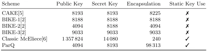
In this section we compare aspects of ParQ’s efficiency and security with other code-based KEMs, many of which have been submitted to NIST’s Post-Quantum Cryptography project [1]. We restrict ourselves to code-based systems for direct comparison. Comparing code-based systems to other post-quantum systems has been done elsewhere in the literature, for example in [5]. All comparisons are done considering parameters that have been proposed for 128 bits of post-quantum security, or NIST’s security level 5 (AES 256) (see table 1).
Scheme Public Key Secret Key Encapsulation Static Key Use
CAKE[5] 8193 8193 8225 7
BIKE-1[2] 8188 8188 8188 7
BIKE-2[2] 4094 8188 4094 7
BIKE-3[2] 9033 9033 9033 7
Classic McEliece[6] 1 357 824 14 080 240 3
ParQ 4094 8193 98 313 3
Table 1: Length in bytes of keys and encapsulations for Code-Based KEMs. Using 8192128 for Classic McEliece
While we do not have specific data on the speed of ParQ as it compares to other systems, one can expect that, because it requires P encapsulations and the decapsulation must be constant time to avoid side-channel timing attacks, the time to encapsulate and decapsulate likely increases by a factor of roughly P as opposed to a construction like CAKE.
be at least 2, note thatP could be set to 1. This would cause the scheme to bear some resemblance to the CAKE scheme [5] or the BIKE-1 scheme [2]. However, this would cause the scheme to be vulnerable to the GJS attack, which is why these schemes currently insist on using the public key ephemerally.
6
Conclusion and Future Work
We have explored and answered several fundamental questions that arose as a result of the powerful GJS reaction attack on QC-MDPC McEliece. We analyzed the origin of this leak: a bias on the distribution of the syndrome weight. This analysis allows a better understanding of the GJS attack and we deduce other side-channel attacks exploiting all decoding instances.
Our analysis provides quantitative bounds on the minimal number of samples needed to deduce relevant information (using Chernoff’s bound), which could be used to deduce better parameters to prevent attacks on the syndrome weight. Other side-channel attacks on different (noisier) parameters exploiting the same idea will be even more costly.
We also discussed how variations in the implemented decoding procedure can affect the attack. Lastly we have showed how decoding failures can be addressed at the protocol level by constructing a KEM that entirely defeats the GJS reac-tion attack for QC-MDPC, without altering the parameters of the system. We provided a proof of the CCA2 security of the KEM in the random oracle model. Notably, this proof considered the possibility of decoding failures, meaning that it should not be possible to attack the system by exploiting decoding failures.
The security of ParQ is proven in the random-oracle model. A complete and thorough analysis of post-quantum security would require a security reduction in the quantum random-oracle model [8]. Showing that ParQ (or a small modifica-tion of ParQ) is secure in this model would give greater post-quantum assurance. MDPC codes are still a recent proposal. Even though they are close to the thoroughly studied LDPC codes, they seem to behave differently, in particular as far as decoding is concerned [9]. It is very likely that the state of the art for decoding MDPC codes will evolve quickly, especially considering the NIST call for quantum safe primitives. Interestingly, it seems that more efficient decoders (e.g. those using variable threshold rules) are more prone to information leakage, and thus better decoders might not be safer. Evaluating new decoding algorithm, their failure rates and running time distribution with respect to this work could indicate whether and at what cost QC-MDPC codes could be used for PKEs as safely as for KEMs.
References
1. NIST post-quantum cryptography project, round 1 submissions (2017),https:// csrc.nist.gov/projects/post-quantum-cryptography/round-1-submissions
E., Sendrier, N., Tillich, J.P., Z´emor, G.: BIKE — bit flipping key encapsulation (2017),http://bikesuite.org
3. Augot, D., Batina, L., Bernstein, D.J., Bos, J., Buchmann, J., Castryck, W., Dunkelman, O., G¨uneysu, T., Gueron, S., H¨ulsing, A., Lange, T., Mohamed, M.S.E., Rechberger, C., Schwabe, P., Sendrier, N., Vercauteren, F., Yang, B.Y.: Initial recommendations of long-term secure post-quantum systems (2015),http: //pqcrypto.eu.org/docs/initial-recommendations.pdf
4. Baldi, M., Bodrato, M., Chiaraluce, F.: A new analysis of the McEliece cryptosys-tem based on QC-LDPC codes. In: Proceedings of Security and Cryptography for Networks, 6th International Conference (SCN 2008). pp. 246–262 (2008)
5. Barreto, P.S.L.M., Gueron, S., G¨uneysu, T., Misoczki, R., Persichetti, E., Sendrier, N., Tillich, J.P.: CAKE: Code-based algorithm for key encapsulation. Cryptology ePrint Archive, Report 2017/757 (2017)
6. Bernstein, D.J., Chou, T., Lange, T., von Maurich, I., Misoczki, R., Niederhagen, R., Persichetti, E., Peters, C., Schwabe, P., Sendrier, N., Szefer, J., Wang, W.: Classic mceliece (2017),https://classic.mceliece.org
7. Bernstein, D.J., Chou, T., Schwabe, P.: McBits: Fast constant-time code-based cryptography. In: CHES 2013. LNCS, vol. 8086, pp. 250–272. Springer (2013) 8. Boneh, D., Dagdelen, ¨O., Fischlin, M., Lehmann, A., Schaffner, C., Zhandry, M.:
Random oracles in a quantum world. In: Asiacrypt 2011. LNCS, vol. 7073, pp. 41–69. Springer (2011)
9. Chaulet, J.: ´Etude de cryptosyst`emes `a cl´e publique bas´es sur les codes MDPC quasi-cycliques. Ph.D. thesis, Universit´e Pierre et Marie Curie-Paris VI (2017) 10. Chaulet, J., Sendrier, N.: Worst case QC-MDPC decoder for mceliece
cryptosys-tem. In: IEEE International Symposium on Information Theory, (ISIT 2016). pp. 1366–1370 (2016)
11. Chen, C., Eisenbarth, T., von Maurich, I., Steinwandt, R.: Differential power analy-sis of a mceliece cryptosystem. In: 13th International Conference on Applied Cryp-tography and Network Security (ACNS 2015) Revised Selected Papers. pp. 538–556 (2015)
12. Chen, C., Eisenbarth, T., von Maurich, I., Steinwandt, R.: Horizontal and ver-tical side channel analysis of a mceliece cryptosystem. IEEE Trans. Information Forensics and Security 11(6), 1093–1105 (2016)
13. Chou, T.: QcBits: Constant-time small-key code-based cryptography. In: CHES 2016. LNCS, vol. 9813, pp. 280–300. Springer (2016)
14. Deneuville, J.C., Gaborit, P., Z´emor, G.: Ouroboros: A simple, secure and efficient key exchange protocol based on coding theory. In: PQCrypto 2017. LNCS, vol. 10346, pp. 18–34. Springer (2017)
15. Dent, A.W.: A designer’s guide to KEMs. In: Cryptography and Coding: 9th IMA International Conference, Proceedings. LNCS, vol. 2898, pp. 133–151. Springer (2003)
16. D¨ottling, N., Dowsley, R., M¨uller-Quade, J., Nascimento, A.C.A.: A CCA2 secure variant of the McEliece cryptosystem. IEEE Transactions on Information Theory 58(10), 6672–6680 (2012)
17. Fabˇsiˇc, T., Hromada, V., Stankovski, P., Zajac, P., Guo, Q., Johansson, T.: A reaction attack on the QC-LDPC McEliece cryptosystem. In: PQCrypto 2017. LNCS, vol. 10346, pp. 51–68. Springer (2017)
18. Gaborit, P.: Shorter keys for code based cryptography. In: Proceedings of WCC 2005. pp. 81–90 (2005)
20. Guo, Q., Johansson, T., Stankovski, P.: A key recovery attack on MDPC with CCA security using decoding errors. In: Asiacrypt 2016. LNCS, vol. 10031, pp. 789–815. Springer (2016)
21. Habib, M., McDiarmid, C., Ramirez-Alfonsin, J., Reed, B.: Probabilistic methods for algorithmic discrete mathematics, vol. 16. Springer Science & Business Media (2013)
22. Heyse, S., von Maurich, I., G¨uneysu, T.: Smaller keys for code-based cryptography: QC-MDPC McEliece implementations on embedded devices. In: Proceedings of the 15th International Workshop on Cryptographic Hardware and Embedded Systems (CHES 2013). pp. 273–292 (2013)
23. Kobara, K., Imai, H.: Semantically secure McEliece public-key cryptosystems-conversions for McEliece PKC. In: Public Key Cryptography 2001. pp. 19–35. PKC ’01, Springer-Verlag (2001)
24. Kocher, P.C.: Timing attacks on implementations of Diffie-Hellman, RSA, DSS, and other systems. In: CRYPTO ’96. LNCS, vol. 1109, pp. 104–113. Springer (1996) 25. von Maurich, I., G¨uneysu, T.: Towards side-channel resistant implementations of QC-MDPC McEliece encryption on constrained devices. In: PQCrypto 2014. LNCS, vol. 8772, pp. 266–282. Springer (2014)
26. von Maurich, I., Heberle, L., G¨uneysu, T.: IND-CCA secure hybrid encryption from QC-MDPC Niederreiter. In: PQCrypto 2016. LNCS, vol. 9606, pp. 1–17. Springer (2016)
27. von Maurich, I., Oder, T., G¨uneysu, T.: Implementing QC-MDPC McEliece en-cryption. ACM Transactions on Embedded Computing Systems (TECS) 14(3), 44:1–44:27 (2015)
28. McEliece, R.J.: A public-key cryptosystem based on algebraic coding theory. Deep Space Network Progress Report 44, 114–116 (1978)
29. Misoczki, R., Tillich, J.P., Sendrier, N., Barreto, P.S.L.M.: MDPC-McEliece: New McEliece variants from moderate density parity-check codes. In: 2013 IEEE Inter-national Symposium on Information Theory. pp. 2069–2073 (2013)
30. Monico, C., Rosenthal, J., Shokrollahi, A.: Using low density parity check codes in the McEliece cryptosystem. In: IEEE International Symposium on Information Theory – ISIT’2000. p. 215. IEEE (2000)
31. Niederreiter, H.: Knapsack type of cryptosystems and algebraic coding theory 15, 19–34 (1986)
32. Rosen, A., Segev, G.: Chosen-ciphertext security via correlated products. In: TCC 2009. LNCS, vol. 5444, pp. 419–436. Springer (2009)
33. Strenzke, F.: A timing attack against the secret permutation in the McEliece PKC. In: PQCrypto 2010. LNCS, vol. 6061, pp. 95–107. Springer (2010)
34. Strenzke, F.: Timing attacks against the syndrome inversion in code-based cryp-tosystems. In: PQCrypto 2013. LNCS, vol. 7932, pp. 217–230. Springer (2013) 35. Strenzke, F., Tews, E., Molter, H.G., Overbeck, R., Shoufan, A.: Side channels in
the McEliece PKC. In: PQCrypto 2008. LNCS, vol. 5299, pp. 216–229. Springer (2008)
36. Yoshida, Y., Morozov, K., Tanaka, K.: Ouroboros: A simple, secure and efficient key exchange protocol based on coding theory. In: PQCrypto 2017. LNCS, vol. 10346, pp. 35–50. Springer (2017)
A
Security Definitions and Games
The IND-CCA2 and OW-CPA games take place between two parties, the challengerC, and the attacker or adversary,A.
Game 1 (IND-CCA2 Challenge).
1. Cobtains (pk, sk)←ParQ.KeyGen(1λ), and sendspktoA.CrunsParQ.Enc(s) with a uniformly randoms, obtainingK0, C. C then generates a uniformly randomK1 ∈ {0,1}λ, and a uniformly random bitb∈ {0,1}.C then sends CandKb toA.
2. A may freely send decapsulation queries C to C. C responds by sending
ParQ.Dec(C) toA. The only exception is thatAmay not send the challenge encapsulationC as a decapsulation query.
3. Eventually,Amust return a bitb0 as a guess for the bitb.Ais said to have won the IND-CCA2 game ifb0=b.
We write A’s ability to win Game 1 as 1/2 +. We call the adversary’s advantage in breaking IND-CCA2 security.
Game 2 (OW-CPA Challenge).
1. C generates (pk, sk)←QCMDPC.KeyGen(1λ). They select a uniformly ran-domx←− {$ 0,1}k ande←− {$ 0,1}n, with ehaving weightt. They then com-putec∗←QCMDPC.Enc(pk, x, e) and sendsc∗ andpkto A.
2. Aperforms some computation on c∗ andpk. Eventually they must produce anx0.Ais said to have won the OW-CPA game ifx0 =x.
B
Choosing the Bit-flipping Thresholds
In standard literature, rules for threshold computation are heuristic and are not available for all parameter sets. To convince that our experiments were fair we describe the rules we used for fixed and variable threshold. We denoted=w/2 the column weight.
Monitoring Strategy: For a given set of parameters, we run the bit-flipping algo-rithm on many random instances and we choose at each iteration the threshold which minimizes the error weight at the end of all flips1. This is possible in a simulation because we know the initial error pattern and we can monitor its evolution. We will refer to this as the “monitoring strategy” and use it as a tool to define the thresholds.
Fixed Thresholds: For a given set of parameters, we run a simulation using the monitoring strategy and we keep track of the threshold values used at the first iteration. The maximum of those values is kept as the fixed threshold, say b0, for the first iteration. We run a second simulation, for which the first threshold is fixed tob0and the monitoring strategy is used for the following iterations. We keep track of the threshold values used at the second iteration. The maximum of those values is kept as the fixed threshold, sayb1, for the second iteration. We repeat this until we reach the maximal expected number of iterations.
1
Variable thresholds: For a given set of parameters, the goal here is to establish a rulebi(σ),i≥0, giving thei-th iteration threshold as a function of the syndrome weight σ. Assuming all b` for ` < i are known, we run a simulation using the functionsb0, . . . , bi−1for the firstiiterations and using the monitoring strategy after that. We keep track of the pairs (σ, b) of syndrome weights and threshold values used at the i-th iteration. For each syndrome weight σ, we define fi(σ) as the average of all thresholds observed. Next, using the least square method, we find the quadratic2 functiong
i(σ) which best approximates all the (σ, fi(σ)) where each (σ, fi(σ)) is weighted by the number of occurrences of the syndrome weight σ. The threshold function for the i-th iteration will bedgi(σ)e. We add the condition thatbi is increasing withσand we getbi :σ→max bmini ,dgi(σ)e
wherebmini is the minimal value ofdgi(σ)eover the observed range forσ, and is never smaller than d/2.
Results and Comments. We give below the threshold rules we used for our simulations deduced from the above-mentioned process. Note that we do not claim, nor observed, that those rules are giving any kind of improvement in speed or failure rate.
Fixed Thresholds. For 80-bit security parameters, (k, w, t) = (4801,90,84), we have (bi)i≥0 = (30,28,26,25,23, . . .). The dots meaning that the last value is repeated as much as necessary. We remark that, for the same parameters, QcBits [13] uses thresholds that are exactly one unit lower for the first 4 iterations. This probably reflects the fact that our strategy is rather conservative.
For 128-bit security, (k, w, t) = (10163,142,134), we get (bi)i≥0= (46,43,41, 40,39,37,36, . . .). Finally for 256-bit security, (k, w, t) = (32771,274,264) we obtain (bi)i≥0= (83,80,77,74,72, . . .).
Variable Thresholds.
(k, w, t) = (4801,90,84) ⇒
b0(σ) =d11.1 + 0.00919σe
b1(σ) = max(24,d38.7−0.0242σ+ 1.004 10−5σ2e) bi(σ) = max(24,d34.9−0.0195σ+ 0.836 10−5σ2e), i≥2,
(k, w, t) =
(10163,142,134) ⇒
b0(σ) =d15.5 + 0.00665σe
b1(σ) =d51.7−0.0128σ+ 0.257 10−5σ2e
bi(σ) = max(37,d40.1−0.00395σ+ 9.50 10−7σ2e, i≥2
(k, w, t) =
(32771,274,264) ⇒
b0(σ) =d22.9 + 0.00402σe b1(σ) =d18.2 + 0.00431σe
b2(σ) = max(71,d315.8−0.0422σ+ 0.182 10−5σ2e) bi(σ) = max(69,d62.5 + 0.000648σe), i≥3.
2