Connecting Legendre with Kummer and Edwards
Sabyasachi Karati iCIS Lab
Department of Computer Science University of Calgary
Canada
e-mail: [email protected]
Palash Sarkar Applied Statistics Unit Indian Statistical Institute
203, B.T. Road, Kolkata India 700108. e-mail: [email protected] December 14, 2017
Abstract
Scalar multiplication on Legendre form elliptic curves can be speeded up in two ways. One can perform the bulk of the computation either on the associated Kummer line or on an appropriate twisted Edwards form elliptic curve. This paper provides details of moving to and from between Legendre form elliptic curves and associated Kummer line and moving to and from between Legendre form elliptic curves and related twisted Edwards form elliptic curves. Further, concrete twisted Edwards form elliptic curves are identified which correspond to known Kummer lines at the 128-bit security level which provide very fast scalar multiplication on modern architectures supporting SIMD operations.
Keywords: Elliptic curve, Legendre form, Edwards form, Kummer line
1
Introduction
Scalar multiplication over an elliptic curve is a basic operation for implementation of basic public key function-alities including Diffie-Hellman key exchange and digital signature schemes. Consequently, secure and efficient algorithms for scalar multiplication are of paramount importance in practical deployment of such schemes. De-pending on the target functionality, it is required to consider various cases of scalar multiplication, namely fixed base scalar multiplication, variable base scalar multiplication and multi-scalar multiplication. Diffie-Hellman key exchange has two phases, the first phase consists of computation of the public key and requires a fixed base scalar multiplication whereas the second phase consists of shared secret computation and requires a variable base scalar multiplication. On the other hand, signature generation requires a fixed base scalar multiplication while signature verification requires multi-scalar multiplication.
Our Contributions:
Connecting Legendre to Kummer: A Kummer line is not a group. In fact, a Kummer line is associated with a Legendre form elliptic curve. A scalar multiplication on the Kummer line does not require they-coordinate of the Legendre curve point. For shared secret computation in Diffie-Hellman computation, it is sufficient to consider only variable base scalar multiplication on the Kummer line. More generally, one may be interested in performing a full scalar multiplication on the Legendre form curve. This requires a method for recovering the y-coordinate of the result from the Kummer line computation. The first contribution of the present paper is to provide a detailed explicit formula for doing this. The earlier work [15] had briefly sketched the method, but, the details provided in the present work were not given in [15].
Connecting Legendre to Edwards: As mentioned above, fixed base scalar multiplication can benefit from the use of suitable twisted Edwards form curve. The fastest known scalar multiplication formula is for special types of twisted Edwards form curves [13]. Our second and main contribution is to provide three conversion methods from Legendre form curves to appropriate twisted Edwards form curves. Two of the conversion methods are birational equivalences while the third one is a 2-isogeny. Each method is built by composing several individual mappings. All of the individual mappings have appeared earlier in the literature. Our contribution is to put together these mappings in an appropriate manner and to supply details which have not been provided in earlier works. We go beyond the task of just providing the mappings and propose concrete twisted Edwards form curves corresponding to the concrete Kummer lines introduced in [15].
The net effect of the present work is to obtain a set of concrete Legendre form curves and associated Kummer lines and twisted Edwards form curves. Scalar multiplication on the Legendre form curves can be done by moving to either the associated Kummer line or to the associated twisted Edwards form curve. The complete details for moving to and from between the Legendre form curves and the associated Kummer lines and for moving to and from between the Legendre form curves and the corresponding twisted Edwards form curves are provided. Depending on the requirement, one may choose to perform scalar multiplication on the Legendre form curve via the Kummer line or via the twisted Edwards form curve. For certain applications, it may also be sufficient to work only on the Kummer line or only on the twisted Edwards form curve.
Previous and Related Works:
Elliptic curve cryptography (ECC) was introduced independently by Koblitz [16] and Miller [17]. Over the years, ECC has become the method of choice for compact and efficient implementation of various public key operations. Montgomery [18] introduced the so-called Montgomery form of elliptic curves which provided a method for very fast x-coordinate only scalar multiplication. The famous Curve25519proposed by Bernstein [2] is based on the Montgomery form elliptic curve. Bernstein and Lange [4] proposed the use of Edwards form curve [9] to cryptography. A later work [5] introduced the twisted Edwards form curve. The fastest known scalar multiplication algorithm for certain types of twisted Edwards form curves was proposed by Hisil et al [13]. Gaudry [11] proposed the use of Kummer surfaces for speeding up scalar multiplication and a later work by Gaudry and Lubicz [12] suggested the use of Kummer lines. As mentioned earlier, this idea was fully developed in [15] where concrete Kummer lines were suggested and implementation and timing results were reported.
2
Kummer Line and Elliptic Curves
A brief background on Kummer lines and the relevant forms of elliptic curves are provided in this section.
2.1 Kummer Line
are used have a good reduction [12] which makes it possible to use the Lefschetz principle [1, 10] to carry over the identities which hold over the complex to those over a large characteristic field.
Letϑ1, ϑ2,Θ1 and Θ2 be functions from CtoCsatisfying the following identities. 2Θ1(w1+w2)Θ1(w1−w2) = ϑ1(w1)ϑ1(w2) +ϑ2(w1)ϑ2(w2);
2Θ2(w1+w2)Θ2(w1−w2) = ϑ1(w1)ϑ1(w2)−ϑ2(w1)ϑ2(w2);
(1)
ϑ1(w1+w2)ϑ1(w1−w2) = Θ1(2w1)Θ1(2w2) + Θ2(2w1)Θ2(2w2);
ϑ2(w1+w2)ϑ2(w1−w2) = Θ1(2w1)Θ1(2w2)−Θ2(2w1)Θ2(2w2).
(2)
For the concrete definition of the theta functions in genus one and the proofs of the above identities, we refer to [15]. For the general theory covering higher genus we refer to [19, 14] and to [11, 12] for proposing cryptographic applications of theta functions.
Puttingw1 =w2 =w in (1) and (2), we obtain
2Θ1(2w)Θ1(0) = ϑ1(w)2+ϑ2(w)2;
2Θ2(2w)Θ2(0) = ϑ1(w)2−ϑ2(w)2;
(3)
ϑ1(2w)ϑ1(0) = Θ1(2w)2+ Θ2(2w)2;
ϑ2(2w)ϑ2(0) = Θ1(2w)2−Θ2(2w)2. (4)
Puttingw= 0 in (3), we obtain
2Θ1(0)2 = ϑ1(0)2+ϑ2(0)2;
2Θ2(0)2 = ϑ1(0)2−ϑ2(0)2. (5)
Denote byP1(C) the projective line overC. Given a2 =ϑ1(0)2 and b2 =ϑ2(0)2, the Kummer line Ka2,b2 is
the image of the map ϕfrom CtoP1(C) defined by
ϕ:w7−→[ϑ1(w) :ϑ2(w)]. (6)
LetA and Bbe such that A2=a2+b2 and B2 =a2−b2. Suppose that P = [x2
1 : z21] is known where x1 = ϑ1(w), z1 = ϑ2(w) and ϕ(w) = [ϑ1(w) : ϑ2(w)] for some
w ∈C. Using (3) and (4) it is possible to compute 2P = [x23 :z23] where x3 =ϑ1(2w) and z3 =ϑ2(2w) without
knowing the value ofw. This procedure is called doubling and Algorithmdblin Table 1 shows how to obtainx23 and z2
3 fromx21 and z21.
Suppose thatP1 = [x21 :z21], P2 = [x22 :z22] andP1−P2 = [x2 :z2] are known, where xi =ϑ1(wi), zi =ϑ2(wi),
i= 1,2; x=ϑ1(w1−w2) and z= ϑ2(w1−w2). Using (1) and (2) it is possible to compute P1+P2 = [x23 :z23]
where x3 = ϑ1(w1 +w2) and z3 = ϑ2(w1+w2). This procedure is called differential (or pseudo) addition and
Algorithm diffAddin Table 1 shows how to obtain x23 and z23 from x21,z21,x22,z22,x2 and z2.
With respect to the above defined doubling and differential addition, the point [a2 :b2] acts as the identity element while the point [b2:a2] has order two. GivenP= [x2
1:z21] on Ka2,b2 and a positive integern, Algorithm
scalarMult in Table 2 returns (R, S), where R=nP= [x2n:z2n] and S= (n+ 1)P= [x2n+1 :z2n+1].
Since both doubling and differential addition work with only squared quantities, this is referred to as the square only setting.
dbl(x2,z2)
s0 =B2(x2+z2)2;
t0 =A2(x2−z2)2;
x23=b2(s0+t0)2;
z23 =a2(s0−t0)2;
return (x23,z23).
diffAdd(x21,z21,x22,z22,x2,z2) s0 =B2(x21+z21)(x22+z22);
t0=A2(x21−z21)(x22−z22);
x23 =z2(s0+t0)2;
z23=x2(s0−t0)2;
return (x23,z23).
Table 1: Double and differential addition in the square-only setting.
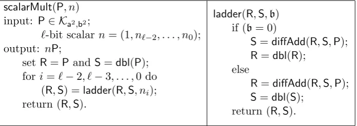
scalarMult(P, n) input: P∈ Ka2,b2;
`-bit scalarn= (1, n`−2, . . . , n0);
output: nP;
setR=P and S=dbl(P); fori=`−2, `−3, . . . ,0 do
(R,S) =ladder(R,S, ni); return (R,S).
ladder(R,S,b) if (b= 0)
S=diffAdd(R,S,P); R=dbl(R);
else
R=diffAdd(R,S,P); S=dbl(S);
return (R,S).
Table 2: Scalar multiplication on Kummer line using a ladder.
2.2 Legendre Form Elliptic Curve
The Legendre form elliptic curve EL,µ in affine coordinates (x, y) is given by an equation
EL,µ:y2 = x(x−1)(x−µ) (7)
withµ∈Fp\{0}. The projective coordinates (X:Y :Z) correspond to the affine point (X/Z, Y /Z). In projective coordinates, the curve has the formEL,µ:Y2Z =X(X−Z)(X−µZ).To avoid introducing additional notation, we will useEL,µ to denote both the affine and the projective forms of the curve. The intended form will be clear from the context. The curveEL,µ has three points of order two, namely, (0 : 0 : 1), (1 : 0 : 1) and (µ: 0 : 1). Let T= (µ: 0 : 1).
LetKa2,b2 be a Kummer line such that
µ = a
4
a4−b4. (8)
Letσ :EL,µ →EL,µ be the automorphism which maps a point of EL,µ to its inverse, i.e., for (X :Y :Z)∈
EL,µ,σ(X:Y :Z) = (X :−Y :Z). An explicit mapψ:Ka2,b2 \ {[b2 :a2]} →EL,µ/σhas been given in [12].
ψ([x2:z2]) =
(1 : 0 : 0) if [x2 :z2] = [a2 :b2];
(a2x2:·:a2x2−b2z2) otherwise; (9)
ψ−1((X:·:Z)) =
[a2 :b2] if (X :·:Z) = (1 :·: 0);
[b2X:a2(X−Z)] otherwise. (10)
The map ψ by itself does not preserve the consistency of doubling and differential addition between EL,µ and Ka2,b2. Instead, the map ψneeds to be extended to obtain a map ψb:Ka2,b2\ {[b2 :a2]} →EL,µ/σwhere
b
The map ψb preserves the consistency of doubling and addition between EL,µ and Ka2,b2. We refer to [15] for
details. Further, it can be argued [12, 15] that the discrete logarithm problem in EL,µ and Ka2,b2 are equally
hard.
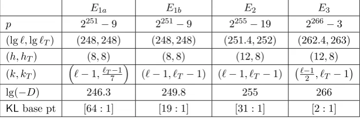
2.3 Concrete Choices of Kummer Lines
For cryptographic purposes, we work over a large characteristic field. As mentioned earlier, since all the identities have good reductions, using the Lefschetz principle, the identities also hold over such finite fields. Further, since the characteristicpof the field will be large and we will choose small values ofa2 and b2,a4−b4 will not be zero modulo pso that µis also defined over Fp.
We consider the following concrete Kummer lines.
KL1a:=KL2519(81,20) : The Kummer line K81,20over the field F2251−9.
KL1b:=KL2519(186,175) : The Kummer line K186,175 over the field F2251−9.
KL2 :=KL25519(82,77) : The Kummer line K82,77over the field F2255−19.
KL3 :=KL2663(260,139) : The Kummer line K260,139 over the field F2266−3.
The work [15] proposedKL1a,KL2andKL3. We additionally considerKL1b. The efficiency of scalar multiplication on KL1b is the same as that of KL1a. On the other hand, for conversion to twisted Edwards form,KL1b provides a few more options which are not obtained from eitherKL1a,KL2 orKL3.
By E1a,E1b,E2 and E3 we will denote the group ofFp-rational points of the Legendre form elliptic curves corresponding toKL1a,KL1b,KL2 and KL3 respectively.
All of the proposals provide security at about the 128-bit level. The relevant properties of these proposals are shown in Table 3. Comparison to other well known proposals are given in [15]. In Table 3, `and `T are the orders of the largest prime subgroups of the curves and their quadratic twists; h andhtare the co-factors of the curves and their quadratic twists; and Dis the complex multiplication field discriminant [3].
Table 3: Some properties of the group ofFp-rational points of the Legendre form elliptic curvesE1a,E1b,E2 and
E3.
E1a E1b E2 E3
p 2251−9 2251−9 2255−19 2266−3
(lg`,lg`T) (248,248) (248,248) (251.4,252) (262.4,263)
(h, hT) (8,8) (8,8) (12,8) (12,8)
(k, kT)
`−1,`T7−1 (`−1, `T −1) (`−1, `T −1) `−21, `T −1
lg(−D) 246.3 249.8 255 266
KL base pt [64 : 1] [19 : 1] [31 : 1] [2 : 1]
2.4 Twisted Edwards Form Elliptic Curve
which corresponds to the extended affine coordinates (U/W, V /W, T /W). The identity element is represented as (0 : 1 : 0 : 1) and the inverse of (U, V, T, W) is (−U :V :−T :W).
Ifa=−1, i.e., the curveEE,−1,d has the currently fastest addition algorithm in the extented twisted Edwards coordinates. So, it is of interest to be able to move fromEE,a,d toEE,−1,d0. Based on the discussion in Section 2
of [5], we have the following two options.
Suppose the Legendre symbolsapand−p1are equal. Thenacan be written asa=−b2 for some b∈Fp. The map
(u, v) 7→ (u, v) = (bu, v) (14)
is an isomorphism over Fp fromEE,a,d :au2+v2= 1 +du2v2 toEE,−1,−d/a:−u2+v2= 1 + (−d/a)u2v2. Suppose
a p
6=−p1but,
d p
=
−1
p
. The map
(ˆu,ˆv) 7→ (u, v) = (ˆu,1/vˆ) (15)
is a birational equivalence overFp from EE,a,d:auˆ2+ ˆv2= 1 +duˆ2vˆ2 toEE,d,a :du2+v2 = 1 +au2v2 having the exceptional point ˆv= 0. One can then apply the map in (14) toEE,d,a to move toEE,−1,−a/d.
Remark: The equation −u2+v2 = 1 +du2v2 can be rewritten as u2(1 +dv2) =v2 −1. If 1 +dv2 = 0, then v2 = 1 and then d = −1. So, if d 6= −1, then 1 +dv2 6= 0 and u = ±p
(v2−1)/(1 +dv2). On the other
hand, if d= −1, then v2 = 1 corresponds to the two points (0,1) (the identity) and (0,−1) (having order 2). In our applications, d6=−1. So, given the value of v and the sign of u, it is possible to uniquely determine u. Following [6], this allows compressing the point (u, v) to (sgn(u), v) which is useful for applications to Edwards curve based signature verification.
2.5 Montgomery form Elliptic Curve
The Montgomery form elliptic curve EM,A,B in affine coordinates (r, s) is given by an equation
EM,A,B:Bs2 = r3+Ar2+r (16)
with A ∈Fp \ {−2,2} and B ∈ Fp\ {0}. We will encounter Montgomery form elliptic curves while transiting from Legendre form curves to Edwards form curves. There will be no occasion to use projective coordinates of the Montgomery form and hence we do not introduce it here.
The connection between Montgomery and twisted Edwards form that we will use is given by Theorem 3.2 of [5]. The Montgomery curve EM,A,B :Bs2 = r3 +Ar2+r is birationally equivalent to the twisted Edwards curve EE,a,d :au2+v2 = 1 +du2v2 with a= (A+ 2)/B and d= (A−2)/Band is given by the map
(r, s) 7→ (u, v) = (r/s,(r−1)/(r+ 1)). (17)
The exceptional points are given by s= 0 and r=−1.
2.6 Weierstrass form Elliptic Curve
The Weierstrass form elliptic curve EW,a,b in affine coordinates (x,y) is given by an equation
EW,a,b :y2 = x3+ax+b (18)
Proposition 1 in [20] shows thatEW,a,b can be converted into a Montgomery form if and only if the following two conditions hold.
1. There is anα∈Fp such that α3+aα+b= 0.
2. For thisα, there is ac∈Fp such thatc2= (3α2+a)−1.
(19)
Suppose that (19) holds. Then the map
(x,y) 7→ (r, s) = (c(x−α),cy) (20)
is an isomorphism from EW,a,b:y2 =x3+ax+btoEM,A,B :Bs2=r3+Ar2+r where A= 3αcand B =c.
2.7 Notation
1. Upper-case bold face letters P,Q,R and S denote points of elliptic curves and upper case letters P,Q,R and Sin sans serif font denote points of Kummer lines.
2. [x2 :z2] denote points on the Kummer line.
3. (x, y) denotes affine Legendre coordinates; (X, Y, Z) denotes projective Legendre coordinates.
4. (u, v, t) denotes extended affine Edwards coordinates; (U, V, T, W) denotes extended twisted Edwards co-ordinates.
5. (r, s) denotes affine Montgomery coordinates.
6. (x,y) denotes affine Weierstrass coordinates.
M,S,A denote multiplication, squaring and addition respectively overFp;C denotes multiplication by a small constant overFp.
3
Moving Between
E
µand
K
a2,b2Suppose P = [x2 : z2] is a point of Ka2,b2 which is not of order two and let ψb(P) = P = (X : · : Z) be the
corresponding point of EL,µ. We wish to obtain formulas for X and Z in terms of x2 and z2. Note that the
Table 4: Conversions from Kummer line to Legendre form elliptic curves and vice versa. Here α0 = a4b2 and
α1=a2b4 are precomputed quantities.
KL to Legendre Legendre to KL
b
ψ([x2 :z2]) X=α0z2;
t1 =α1x2;
t2 =α0z2;
Z=t2−t1;
return (X:·:Z).
b
ψ−1(X:·:Z)
x2 =α0(X−Z);
z2 =α1X;
return [x2:z2].
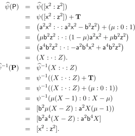
P= [x2:z2]. These tasks are done as follows.
b
ψ(P) = ψb([x2:z2])
= ψ([x2:z2]) +T
= a2x2 :·:a2x2−b2z2+ (µ: 0 : 1) = µb2z2 :·: (1−µ)a2x2+µb2z2 = a4b2z2 :·:−a2b4x2+a4b2z2
= (X :·:Z). (21)
b
ψ−1(P) = ψb−1(X:·:Z)
= ψ−1((X:·:Z) +T)
= ψ−1((X:·:Z) + (µ: 0 : 1)) = ψ−1(µ(X−1) : 0 :X−µ) = [b2µ(X−Z) :a2X(µ−1)) = [b2a4(X−Z) :a2b4X]
= [x2 :z2]. (22)
Explicit formulas to compute the expressions given by (21) and (22) are shown in Table 4. We note that the expressions given by (21) and (22) and the formulas appearing in Table 4 do not appear in [15]. Sincea2 and b2 are small constants, the pre-computed constantsα0 andα1 are also not too large. The conversion from Kummer
line to Legendre form elliptic curve requires three multiplications by small constants while the conversion from Legendre form elliptic curve to Kummer line requires two such multiplications.
UsingΨ, it is possible to map theb KL base points provided in Table 3 to base points on the corresponding
Legendre form curves. These are shown in affine coordinates in Table 5. For the Legendre form curves, the y-coordinate is the positive square root ofx(x−1)(x−µ) where x=a4b2z2/(−a2b4x2+a4b2z2) for the values
of a2,b2,x2 and z2 shown in Table 5. These values are as follows.
y1 = 660779751606431880601449706469571005138317100501546769210310679914171628271,
y2 = 1013622307264833457094516843375813280991440301524377584697694137170779641791,
y3 = 42555777381561203390446781614530346580731893768994719503541652642429650485645,
Table 5: Base points forE1a,E1b,E2 and E3 corresponding to KL1a,KL1b,KL2 and KL3.
p a2 b2 [x2 :z2] (x, y)
2251−9 81 20 [64 : 1] (−131220/1942380,y1)
2251−9 186 175 [19 : 1] (−6054300/102174450,y 2)
2255−19 82 77 [31 : 1] (−504300/13794450,y 3)
2266−3 260 139 [2 : 1] (−9396400/650520,y4)
3.1 Scalar Multiplication on Eµ via Ka2,b2
The main purpose of using Kummer lines is to be able to perform fast scalar multiplication. SupposeP= (XP :
YP : ZP) is a point on EL,µ and n is a positive integer. The requirement is to obtain Q = nP. Using the associated Kummer lineKa2,b2, this is achieved in the following manner.
Set P = ψb−1(P) and compute (Q,R) = scalarMult(P, n). Then Q = nP and R = (n+ 1)P. Set Q =ψb(Q)
and R=ψb(R). By the consistency of scalar multiplication betweenKa2,b2 and EL,µ, it follows thatQ=nPand
R= (n+ 1)P. LetQ= (XQ:YQ:ZQ) andR= (XR:YR:ZR).
The problem with the above approach is that Q = ψb(Q) does not recover YQ. On the other hand, since
Q−R=−P, the value ofYQ can be recovered from XP ,YP,ZP,XQ,ZQ,XRand ZR. The method for doing this has been mentioned in [15] in the context of affine coordinates. Here we solve a more general problem in projective coordinates.
Given Q = (x2Q :z2Q), R= (x2R : zR2) and P = (XP : YP :ZP), we provide formulas for determining XQ, YQ and ZQ. We assume thatPis not the identity nor a point of order two, so thatZP 6= 0 andYP 6= 0. Let
γQ =µb2z2Q, δQ = (1−µ)a2x2Q+µb2z2Q;
γR=µb2z2R, δR = (1−µ)a2x2R+µb2z2R. Then
b
ψ(Q) =ψb([x2Q:zQ2]) = (γQ :·:δQ) =Q and ψb(R) =ψb([x2R :zR2]) = (γR :·:δR) =R.
For simplicity of the ensuing calculation, we shift to affine coordinates. Pin affine coordinates is (xP, yP) where
xP = XP/ZP and yP = YP/ZP. Let xQ = γQ/δQ and xR = γR/δR and so Q and R in affine coordinates are (xQ, yQ) (withyQ unknown) and (xR,·) respectively.
Since Q = nP and R = (n+ 1)P, Q 6= R and so Q 6= R implying that xQ 6= xR. Further, Q = nP and R = (n+ 1)P and so Q−R = −P. Let y = mx+c be the line passing through Q and −R. This line also passes through P and so we havem = (yQ−yP)/(xQ−xP). Plugging the equation y =mx+c into the affine form of the curve y2 =x3−(µ+ 1)x2+µx and simplifying we have x3−(µ+ 1 +m2)x2+ (µ−2mc)x−c2= 0. Since xP,xQ andxRare the three roots of this equation, we havexP+xQ+xR=µ+ 1 +m2. Substituting the expression for m and using y2Q=xQ(xQ−1)(xQ−µ) we obtain
yQ=− 1 2yP
(xQ−xP)2(xP +xQ+xR−µ−1)−xQ(xQ−1)(xQ−µ)−y2P
Substituting xQ =γQ/δQ,xR=γR/δR,xP =XP/ZP and yP =YP/ZP, yields yQ
= −ZP
2YP
γ
Q
δQ
−XP
ZP
2X
P
ZP
+γQ δQ
+γR δR
−µ−1
−γQ
δQ
γ
Q
δQ
−1 γQ δQ −µ − Y 2 P Z2 P ! = · · ·
= −1
2YPδQ3δRZP2
(ZPγQ−XPδQ)2(XPδQδR+ZPγQδR+ZPδQγR−(µ+ 1)ZPδQδR)
−ZP3δRγQ(γQ−δQ)(γQ−µδQ)−YP2δ 3
QδRZP
.
Converting back to projective coordinates, using µ= a4/(a4 −b4) and defining pre-computed constants β0 =
2a4−b4 and β1 =a4−b4 we have
Q= [xQ:yQ: 1] = (XQ:YQ:ZQ)
where
XQ = 2γQYPδ2QδRZP2β1,
YQ = − (ZPγQ−XPδQ)2(β1(XPδQδR+ZPγQδR+ZPδQγR)−β0ZPδQδR) −ZP3δRγQ(γQ−δQ)(β1γQ−a4δQ)−YP2δQ3δRZPβ1
, ZQ = 2YPδQ3δRZP2β1.
(23)
The computations ofXQ, YQ andZQ are shown in Algorithm 1. The total cost is 4C+ 26M+ 4S+ 10A.
4
Moving From Legendre to Twisted Edwards Form Elliptic Curves
The general idea is to move from the Legendre form to the Montgomery form and then use (17) to move to the twisted Edwards form. Further, we wish to move toEE,−1,dfor somed. For this, we use either (14) directly or (15) followed by (14) whenever these are feasible to be applied. For moving from the Legendre to the Montgomery form we identify three approaches.
1. If the curve has a point of order 4, then the method given in [4] can be simplified to move from the Legendre form to the Montgomery form. This provides a birational equivalence between the two forms.
2. It is possible to move from the Legendre form to the Weierstrass form. Then using (20) it is possible to move to the Montgomery form, if feasible. This also provides a birational equivalence between the two forms.
3. Based on the method provided in [5], it is possible to obtain a 2-isogeny for moving from the Legendre form to the Montgomery form.
Algorithm 1 Compute Q = (XQ :YQ :ZQ) from P = (XP, YP, ZP), Q = [x2Q : z2Q] and R = [x2R :z2R] where Q=nP,Q=nP,R= (n+ 1)P andP=ψb−1(P). Hereβ0= 2a4−b4,β1=a4−b4,β2 =µb2 andβ3= (1−µ)a2.
A multiplication by µis counted as a general multiplication overFp.
1: Input: P= (XP :YP :ZP),Q= [xQ2 :z2Q],R= [x2R :z2R].
2: Output: Q= (XQ :YQ :ZQ).
3: γQ =β2z2Q;δQ =γQ+β3x2Q; /∗2M+ 1A ∗/
4: γR =β2z2R;δR=γR+β3x2R; /∗2M+ 1A ∗/ 5: t1 ←γQ·ZP; t2 ←XP ·δQ; /∗2M ∗/
6: t3 ←t1−t2; t3 ←t23; /∗1A+ 1S ∗/ 7: t4 ←t1+t2; t4 ←t4·δR; /∗1A+ 1M ∗/
8: t5 ←ZP ·δQ; t6 ←t5·γR; /∗2M ∗/
9: t6 ←t4+t6; t7 ←t5·δR; /∗1A+ 1M ∗/
10: t8 ←β0·t7; t6 ←β1·t6; /∗2C ∗/
11: t6 ←t6−t8; t3 ←t3·t6; /∗1A+ 1M ∗/ 12: t9 ←ZP2; t10←ZP ·δR; /∗1S+ 1M ∗/
13: t11←t9·t10; t12←t11·γQ; /∗2M ∗/
14: t13←γQ−δQ; t14←δQ·a4; /∗1A+ 1C ∗/
15: t6 ←β1·γQ; t14←t6−t14; /∗1A+ 1M ∗/ 16: t12←t12·t13; t12←t12·t14; /∗2M ∗/ 17: t3 ←t3−t12; t15←YP2; /∗1A+ 1S ∗/ 18: t16←t15·δQ2; t17←t16·δQ; /∗2M+ 1S ∗/
19: t18←t10·t17; t18←t18·β1; /∗2M ∗/ 20: t3 ←t18−t3; t19←t10·t16; /∗1A+ 1M ∗/ 21: t19←t19·YP; t19←2β1·t19; /∗1M+ 1C ∗/ 22: t20←t1·t19; t5←t5·t19; /∗2M ∗/ 23: t5 ←t5·ZP; /∗1M ∗/
4.1 Method 1: via a Point of Order 4
Proposition 1. Let Gbe a finite cyclic group of order2iq withq odd and having three points of order two. Then G has a point of order four if and only if i >2.
Proof. If i= 0 or 1, then clearly Gcannot have any point of order 4 as that would violate Lagrange’s theorem. So, supposei≥2. Ifi= 2, then by Sylow’s theoremGhas a unique subgroup of order 4. This subgroup consists of the three points of order 2 along with the identity. So,Gdoes not have any point of order 4. Ifi >2, then by Sylow’s theorem consider the (unique) subgroup H of G of order 2i. The order of any element of H is a power of 2. Since G has three elements of order 2 and the order ofH is at least 8, H must have an element h whose order is 2j forj≥2. The elementh2j−2 is an element of order 4.
From Table 3, the co-factors of E1a,E1b, E2 and E3 are 8, 8, 12 and 12 respectively. Using Proposition 1,
E1a and E1b have points of order 4 whileE2 andE3 do not. The next proposition shows how to find a point of
order 4 in E1a orE1b.
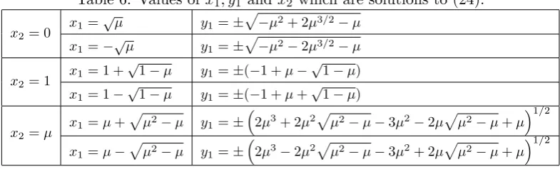
Proposition 2. Consider EL,µ:y2 =x(x−1)(x−µ). The point (x1, y1) is of order 4 if and only if x1 and y1
are solutions of the equations
x3
1−3x2x21+ (2(µ+ 1)x2−µ)x1−µx2 = 0
2y12−(3x21−2(µ+ 1)x1+µ)(x1−x2) = 0
(24)
for some x2 ∈ {0,1, µ} andx16=x2.
Proof. The three points of order 2 onEL,µare (0,0), (1,0) and (µ,0). Since (x1, y1) is a point of order 4, 2(x1, y1)
is a point of order 2 and so is equal to (x2,0) for somex2 ∈ {0,1, µ}.
Letm be the slope of the tangent to the curve passing through the point (x1, y1). This tangent also passes
through the point (x2,0). This gives two ways of obtaining m.
m = 3x
2
1−2(µ+ 1)x1+µ
2y1
= y1−0 x1−x2
.
This shows
2y21 = (x1−x2)(3x21−2(µ+ 1)x1+µ) (25)
= 3x31−2(µ+ 1)x21+µx1−x2(3x21−2(µ+ 1)x1+µ). (26)
Since (x1, y1) is also on the curve,y12 =x13−(µ+ 1)x21+µx1. Substituting in (26) and simplifying we obtain
x31−3x2x21+ (2(µ+ 1)x2−µ)x1−µx2 = 0. (27)
Equations (25) and (27) show the desired result.
Conversely, suppose (24) holds and suppose that 2(x1, y1) = (x2, y2). We need to argue that y2 = 0 which
would imply that (x2, y2) is a point of order 2 and so (x1, y1) is a point of order 4. The slope of the tangent to the
curve at the point (x1, y1) is (3x21−2(µ+ 1)x1+µ)/(2y1) and this tangent also passes through the point (x2, y2).
The line passing through (x1, y1) and (x2, y2) has slope (y1−y2)/(x1−x2). So, (3x21−2(µ+ 1)x1+µ)/(2y1) =
(y1−y2)/(x1−x2). On the other hand, the second equation of (24) shows that (3x21−2(µ+ 1)x1+µ)/(2y1) =
y1/(x1−x2). Comparing the two expressions, we obtainy2 = 0 as required.
Proposition 2 shows a method to find a point of order 4 over Fp. For each value of x2 = 0,1, µ try to
Table 6: Values ofx1, y1 and x2 which are solutions to (24).
x2= 0
x1= √
µ y1=± p
−µ2+ 2µ3/2−µ
x1=− √
µ y1=± p
−µ2−2µ3/2−µ
x2= 1
x1= 1 + √
1−µ y1=±(−1 +µ− √
1−µ) x1= 1−
√
1−µ y1=±(−1 +µ+ √
1−µ)
x2=µ
x1=µ+ p
µ2−µ y 1=±
2µ3+ 2µ2p
µ2−µ−3µ2−2µp
µ2−µ+µ1/2
x1=µ− p
µ2−µ y 1=±
2µ3−2µ2p
µ2−µ−3µ2+ 2µp
µ2−µ+µ1/2
a method different from Proposition 1 of determining whether there is an Fp rational point of order 4. The possible solutions for (x1, y1) arising from solving (24) are given in Table 6. These 12 solutions along with the
3 points of order 2 and the identity provide the 16 elements of the 4-torsion subgroup of EL,µ in the algebraic closure ofFp. Not all of the solutions in Table 6 are inFp.
ForE1a, there are noFp rational points of order 4 corresponding tox2 = 0 andx2 = 1. Forx2 =µ, the point
(µ−pµ2−µ,2µ3−2µ2p
µ2−µ−3µ2+ 2µp
µ2−µ+µ1/2)
is anFp rational point of order 4 such that 2(x1, y1) = (µ,0). The actual values of x1 and y1 are as follows.
x1 = 3224408425544077224047459359771631097399226058139743429316578762596590862491;
y1 = 3138699230617545368821670928998916873427882467813600463343503331843351071540.
ForE1b, there are noFp rational points of order 4 corresponding tox2= 0. For x2 = 1, the point
(1 +p1−µ,−1 +µ−p1−µ)
is anFp rational point of order 4 such that 2(x1, y1) = (1,0). The actual values of x1 and y1 are as follows.
x1 = 2927148786553203617551507184089760902982149768188685673243033378309061916173;
y1 = 1490504580219247555118098514428551370946433127012660449138690111290242828335.
The work [4] proposed the use of Edwards form elliptic curve in cryptography. This work showed birational equivalence between (long) Weierstrass form curves satisfying certain properties and Edwards form curves. From the proof it is possible to pick out a birational equivalence between curves of the form y2 = x3+a2x2+a4x
Lemma 1. [4] Suppose the curve given by E : y2 = x3 +a2x2 +a4x has a point (x1, y1) of order 4 and let
2(x1, y1) = (x2,0). Let E :y2 =x3+A2x2+A4x where A2=a2+ 3x2 and A4 =a4+ 3x22+ 2a2x2. The map
(x, y) 7→ (x, y) = (x−x2, y) (28)
fromE toE is an isomorphism. Further, the point(x1, y1) = (x1−x2, y1)has order4inE and2(x1, y1) = (0,0).
Proof.
y2=y2 = x3+a2x2+a4x.
= (x+x2)3+a2(x+x2)2+a4(x+x2)
= x3+ (a2+ 3x2)x2+ (a4+ 3x22+ 2a2x2)x+x32+a2x22+a2r2
= x3+A2x2+A4x.
The last equation follows from the definition of A2 and A4 and from the fact that (x2,0) is on E. Using [21]
we have that the map given by (28) is an isomorphism. So, it preserves the orders of points. Since (x1, y1) is
mapped to (x1−x2, y1) and (x2,0) is mapped to (0,0), it follows that on E, (x1−x2, y1) is a point of order 4
and 2(x1−x2, y1) = (0,0).
Lemma 2. Suppose the curve given by E:y2=x3+A
2x2+A4x has a point (x1, y1) of order 4 and2(x1, y1) =
(0,0). Then A4 =x21 and A2 =y21/x21−2x1. Further, the map
(x, y) 7→ (r, s) = (x/x1,2y/y1) (29)
is a birational equivalence from E to Bs2 = r3 +Ar2 +r where B = 1/(1−θ) and A = 2(1 +θ)/(1−θ) with θ= 1−4x13/y21.
Proof. The proof is essentially similar to the proof of Theorem 2.1 of [4] with a small difference which we point out later. Since (x1, y1) has order 4,y1 6= 0 and sox16= 0. The point (x1, y1) is onE and so
y2 = x3+A2x2+A4x. (30)
Since 2(x1, y1) = (0,0), the tangent to E at the point (x1, y1) passes through the point (0,0). Following the
proof of Proposition 2, the slope of the tangent can be expressed in two different ways. This yields
y1−0 x1−0
= 3x
2
1+ 2A2x1+A4
2y1
⇒2y21 = 3x31+ 2A2x21+A4x1
⇒2(x31+A2x21+A4x1) = 3x31+ 2A2x21+A4x1 using (30)
⇒A4=x21 sincex16= 0
⇒A2=
y21 x2 1
−2x1 from (30).
From (29), x = rx1 and y = sy1/2. Using y2 = x3 +A2x2 +A4x; the expressions for A2, A4 and θ; and
y21= 4x31/(1−d) we compute as follows.
s2y21 4 =y
2 = x3+A
2x2+A4x=r3x31+A2r2x21+A4rx1
s2x31
1−θ = r
3x3 1+
4 1−θ −2
x31r2+x31r
Remarks:
1. Note that x1/(1−θ) =y21/(4x21) which is a square. This was overlooked in the proof of Theorem 2.1 in [4]
leading to some unnecessary complications.
2. We note that Theorem 3.3 of [5] shows that every elliptic curve having a point of order 4 is birationally equivalent to an Edwards curve and Theorem 3.4 of [5] shows that ifp≡3 mod 4, then every Montgomery curve is birationally equivalent to an Edwards curve. These results are not directly useful for us since we wish to move to a twisted Edwards curve of the form EE,−1,d while these result show how to move to an Edwards curve of the formEE,1,d.
By putting together the different maps, we obtain the following result.
Theorem 3. Let EL,µ : y2 = x(x −1)(x−µ) have a point (x1, y1) of order 4 with 2(x1, y1) = (x2,0). Let
θ = 1−4(x1 −x2)3/y12 and suppose that both −1 and θ are non-squares in Fp. Let 4θ= −b2 for some b∈Fp.
Then EL,µ is birationally equivalent to EE,−1,d : −u2 +v2 = 1 +du2v2 where d = −1/θ and the birational
equivalence is given by
(x, y) 7→ (u, v) =
b(x−x2)y1
(x1−x2)y
,x+x1−2x2 x−x1
(31)
with exceptional points given by y(x−x1) = 0, corresponding to points of order 2 (for y = 0) or to a point of
order 4 (forx=x1). Further, the birational equivalence from EE,−1,d :−u2+v2 = 1 +du2v2 toEL,µ is given by
(u, v) 7→ (x, y) =
x2+ (x1−x2)
v+ 1 v−1,
by1(v+ 1)
2u(v−1)
(32)
with exceptional points given by u(v−1) = 0, corresponding to the identity (0,1) or to the point of order 2 (0,−1).
Proof. EL,µ can be written asy2 =x3+a2x2+a4x where a2 =−(µ+ 1) anda4 =µ. The composition of (28)
and (29) gives the map
(x, y) 7→ (r, s) =
x−x2
x1−x2
, y y1
(33)
which is a birational equivalence from EL,µ to EM,A,B : Bs2 = r3 +Ar2 +r where B = 1/(1−θ) and A = 2(1 +θ)/(1−θ). Composing (33) with (17) and (15) gives the map
(x, y) 7→ (u, v) =
(x−x2)y1
(x1−x2)y
,x+x1−2x2 x−x1
(34)
which is a birational equivalence fromEL,µ toEE,a,4 :au2+v2 = 1 + 4u2v2 wherea= 4θ. Since bothθ and−1
are non-squares inFp,−ais a square and we can writea= 4θ=−b2 for someb∈Fp. Composing (34) with (14) we obtain the map given by (31) which is a birational equivalence from EL,µ toEE,−1,d :−u2+v2 = 1 +du2v2 whered=−1/θ.
Proposition 3. Let µ∈Fp\ {0} and EL,µ:y2 =x(x−1)(x−µ) be in the Legendre form. Let ω= (µ+ 1)/3.
Then the map
(x, y) 7→ (x,y) = (x−ω, y) (35)
is a birational equivalence from EL,µ to EW,a,b :y2 =x3+ax+b where a=µ−3ω2 and b=ω3+ω(µ−2ω2).
Proof. The following computation shows the result.
y2=y2 = x3−(µ+ 1)x2+µx
= (x+ω)3−3ω(x+ω)2+µ(x+ω)
= x3+ 3x2ω+ 3xω2+ω3−3ωx2−6xω2−3ω3+µx+µω = x3+ω3+ (µ−3ω2)x+ω(µ−2ω2)
= x3+ax+b.
Theorem 4. Let µ ∈ Fp \ {0}, ω = (µ+ 1)/3, a = µ−3ω2 and b = ω3 +ω(µ−2ω2). Suppose that α ∈ {−ω,1−ω, µ−ω} is such that c2= (3α2+a)−1 for some c∈Fp. Let a= (3αc+ 2)/cand d= (3αc−2)/c.
1. Suppose that pa=−p1. Then the map
(x, y) 7→ (u, v) =
b(x−ω−α)
y ,
c(x−ω−α)−1
c(x−ω−α) + 1
(36)
is a birational equivalence fromEL,µ:y2=x(x−1)(x−µ)toEE,−1,d:−u2+v2= 1 +du2v2 wherebis such
thata=−b2 andd= (2−3αc)/(2+3αc). The exceptional points of (36) are given byy(c(x−ω−α)+1) = 0.
The converse birational equivalence from EE,−1,d:−u2+v2 = 1 +du2v2 to EL,µ:y2 =x(x−1)(x−µ) is
given by
(u, v) 7→ (x, y) =
α+ω+ 1 +v
c(1−v), b
cu 1 +v 1−v
(37)
with the exceptional points given by u(v−1) = 0.
2. Suppose that pa6=−1
p
and dp=−p1. Then the map
(x, y) 7→ (u, v) =
b(x−ω−α)
y ,
c(x−ω−α) + 1
c(x−ω−α)−1
(38)
is a birational equivalence fromEL,µ:y2=x(x−1)(x−µ)toEE,−1,d:−u2+v2= 1 +du2v2 wherebis such
thatd=−b2 andd= (2+3αc)/(2−3αc). The exceptional points of (38) are given byy(c(x−ω−α)+1) = 0.
The converse birational equivalence from EE,−1,d:−u2+v2 = 1 +du2v2 to EL,µ:y2 =x(x−1)(x−µ) is
given by
(u, v) 7→ (x, y) =
α+ω+ v+ 1
c(v−1), b
cu v+ 1 v−1
(39)
Proof. From Proposition 3, the map (x, y) 7→ (x,y) = (x−ω, y) moves from EL,µ : y2 = x(x−1)(x−µ) to
EW,a,b :y2=x3+ax+b. The conditions onαandcsatisfy (19) fora=µ−3ω2 andb=ω(µ−2ω2). So, from (20) the map (x,y) = (r, s) = (c(x−α),cy) is a birational equivalence from EW,a,b to EM,A,B :Bs2 =r3+Ar2+r whereA= 3αcand B =c.
Suppose that a p = −1 p
. The map (17) given by (r, s) 7→ (u, v) = (r/s,(r−1)/(r+ 1)) is a birational
equivalence from EM,A,B toEE,a,d :a u2+v2 = 1 +du2v2 where a= (A+ 2)/B =a and d= (A−2)/B = d. Using (14), the map (u, v)7→ (u, v) = (bu, v) is a birational equivalence from EE,a,d :a u2+v2 = 1 +du2v2 to EE,−1,d. Composing all the above maps gives the map defined in the first point of the theorem statement.
Suppose that
a
p
6=−p1 and
d p = −1 p
. As above, The map (17) given by (r, s) 7→(ˆu,vˆ) = (r/s,(r−
1)/(r+ 1)) is a birational equivalence from EM,A,B toEE,ˆa,dˆ: ˆauˆ2+ ˆv2 = 1 + ˆduˆ2ˆv2 where ˆa= (A+ 2)/B =a
and ˆd = (A−2)/B = d. Using (15), the map (ˆu,vˆ) 7→ (u, v) = (ˆu,1/vˆ) is a birational equivalence from EE,ˆa,dˆ: ˆauˆ2 + ˆv2 = 1 + ˆduˆ2vˆ2 to EE,a,d :a u2+v2 = 1 +du2v2, where a= ˆd =d and d= ˆa= a. Using (14),
the map (u, v) 7→ (u, v) = (bu, v) is a birational equivalence from EE,a,d : a u2 +v2 = 1 +du2v2 to EE,−1,d. Composing all the maps gives the map defined in the second point of the theorem statement.
4.3 Method 3: via a 2-Isogeny
The statement and proof of the following result is similar to Theorem 5.1 of [5]. We provide more details and more importantly, the final form of the twisted Edwards curve is also different.
Theorem 5. Let µ∈Fp\ {0} and EL,µ:y2 =x(x−1)(x−µ) be a Legendre form curve.
1. If p≡3 mod 4 and µis a non-square in Fp, then the map
(x, y) 7→ (u, v) =
by µ−x2,
y2+x2(1−µ) y2−x2(1−µ)
(40)
is a 2-isogeny fromEL,µ toEE,−1,d :−u2+v2= 1 +du2v2, where b is such that b2 =−4µand d=−1/µ.
The dual 2-isogeny is given by the map
(u, v) 7→ (x, y) =
−µ u2 ,
b(1−µ)v 2u(1−v2)
. (41)
2. If p≡1 mod 4 then the map
(x, y) 7→ (u, v) =
by µ−x2,
y2−(1−µ)x2 y2+ (1−µ)x2
(42)
is a 2-isogeny from EL,µ to EE,−1,d :−u2+v2 = 1 +du2v2, where b is such that b2 = −4 and d= −µ.
The dual 2-isogeny is given by the map
(u, v) 7→ (x, y) =
−1 u2,
(1−µ)bv 2u(v2−1)
and the dual 2-isogeny fromE toEL,µ is given by
(x, y) 7→ (x, y) =
y2 4x2,
y((µ−1)2−x2) 8x2
. (45)
The map
(x, y) 7→ (r, s) = (x/(1−µ), y/(1−µ)) (46)
is an isomorphism from E toEM,A,B :Bs2 =r3+Ar2+r, whereB = 1/(1−µ) and A= 2(1 +µ)/(1−µ). Suppose p ≡ 3 mod 4 and µ is a non-square in Fp. In this case, −1 is a non-square in Fp. Using (17), we obtain a birational equivalence fromEM,A,B toEE,4,4µ: 4ˆu2+ ˆv2 = 1 + 4µuˆ2vˆ2. Using (15), there is a birational equivalence from EE,4,4µ toEE,4µ,4 : 4µu2+v2 = 1 + 4u2v2. Since both −1 and µ are non-squares, using (14),
there is a birational equivalence fromEE,4µ,4toEE,−1,d:−u2+v2= 1+du2v2whered=−1/µ. The intermediate maps for moving from EL,µ toE−1,d are as follows:
(x, y) 7→ (x, y) =
y2 x2,
y(µ−x2) x2
(x, y) 7→ (r, s) =
x 1−µ,
y 1−µ
(r, s) 7→ (ˆu,vˆ) =
r s,
r−1 r+ 1
(ˆu,vˆ) 7→ (u, v) =
ˆ u,1 ˆ v
(u, v) 7→ (u, v) = (bu, v).
Composing these intermediate maps shows that the 2-isogeny fromEL,µ toE,−1,d is given by (40) and composing the maps in the opposite directions shows that the dual 2-isogeny is given by (41).
Supposep≡1 mod 4. In this case,−1 is a square inFp. Using (17), we obtain a birational equivalence from EM,A,B to EE,4,4µ : 4u2 +v2 = 1 + 4µu2v2. Since 4 and −1 are both square, using (14), there is a birational equivalence from EE,4,4µ to EE,−1,d :−u2+v2 = 1 +du2v2 where d=−µ. The intermediate maps for moving from EL,µ toE−1,d are as follows:
(x, y) 7→ (x, y) =
y2 x2,
y(µ−x2) x2
(x, y) 7→ (r, s) =
x 1−µ,
y 1−µ
(r, s) 7→ (u, v) =
r s,
r−1 r+ 1
(u, v) 7→ (u, v) = (bu, v).
Composing these intermediate maps shows that the 2-isogeny fromEL,µ toE,−1,d is given by (42) and composing the maps in the opposite directions shows that the dual 2-isogeny is given by (43).
Corollary 1. Suppose EL,µ is given by projective coordinates (X : Y : Z) and EE,−1,d is given by extended
1. If p≡3 mod 4 and µis a non-square in Fp, then the maps (40) and (41) are respectively (X:Y :Z) 7→ (U :V :T :W)
= bY Z(Y2−X2(1−µ)) : (µZ2−X2)(Y2+X2(1−µ)) :U V : (µZ2−X2)(Y2−X2(1−µ))
(47)
(U :V :T :W) 7→ (X :Y :Z)
= −2µW2(W2−V2) :b(1−µ)U V W2
: 2U2(W2−V2). (48)
2. If p≡1 mod 4, then the maps (42) and (43) are respectively
(X:Y :Z) 7→ (U :V :T :W)
= bY Z(Y2+X2(1−µ)) : (µZ2−X2)(Y2−X2(1−µ))
:U V : (µZ2−X2)(Y2+X2(1−µ)) (49) (U :V :T :W) 7→ (X :Y :Z)
= −2W2(V2−W2) :b(1−µ)U V W2
: 2U2(V2−W2). (50)
Remarks: In the extended twisted Edwards coordinates, the point (0 : 1 : 0 : 1) is the identity and (0 :−1 : 0 : 1) is a point of order 2. In the projective coordinates for Legendre form, the identity is given by (X :Y : 0). The kernels of the isogenies given by (47), (48), (49) and (48) are as follows.
1. For the map (47), the kernel is obtained by setting the right hand side to (0 : 1 : 0 : 1). This leads to the equationsY Z(Y2−X2(1−µ)) = 0, (µZ2−X2)(Y2+X2(1−µ)) = 1 and (µZ2−X2)(Y2−X2(1−µ)) = 1. From the first equation we have eitherZ = 0 orY = 0 orY2−X2(1−µ) = 0. The last condition contradicts the third equation. So, we have eitherZ = 0 or Y = 0. The point corresponding to Z = 0 is the identity of the Legendre form curve. If Z 6= 0, thenY = 0 which corresponds to a point of order 2. The points of order 2 are (0 : 0 : 1), (1 : 0 : 1) and (µ : 0 : 1) and so µZ2−X2 6= 0. So, the last two equations lead to Y2+X2(1−µ) =Y2−X2(1−µ) which combined withY = 0 leads to X= 0. So, the two points in the kernel of (47) are the identity and the point (0 : 0 : 1) of order 2.
2. For the map (41), the kernel is obtained by setting the last component of the right hand side to 0, i.e., U2(W2 −V2) = 0. Suppose U = 0, then from the projective form of the twisted Edwards curve, we have W2(V2−W2) = 0 which using W 6= 0 leads to V = ±W. On the other hand, if W2 −V2 = 0, then from the projective form of the twisted Edwards curve, we have (1 +d)U2 = 0 (using W 6= 0) and so U = 0. So, the points in the kernel are given by U = 0 and V = ±W, i.e., the kernel consists of {(0 : 1 : 0 : 1),(0 :−1 : 0 : 1)}. The first point is the identity of the twisted Edwards curve while the second point has order two.
3. A reasoning similar to the above shows that the kernel of (49) is the same as the kernel of (47) and the kernel of (50) is the same as the kernel of (48).
So, only the parameter dneeds to be determined.
Case 1a: EE,−1,d arising from E1a=EL,µ arising from KL2519(81,20). In this case p= 2251−9 and−1 is a non-square modulo p.
1. Consider the applicability of Theorem 3. This requires a point (x1, y1) of order 4 such that 2(x1, y1) =
(x2, y2) where the possible values of x1, y1 and x2 are given in Table 6. For the solutions ofx1, y1 and x2,
it is required to determine whether theθ defined in Theorem 3 is a non-square. It turns out that for E1a none of the solutions for x1, y1 and x2 lead to a non-square θ. So, Theorem 3 does not lead to a desired
twisted Edwards curve corresponding toE1a.
2. Consider the applicability of Theorem 4. Recall thatω = (µ+ 1)/3,a=µ−3ω2. The choices ofα= 1−ω andα=µ−ωdo not lead to any solution. Forα=−ω, 3α2+ais a square; for both values ofc=±√3α2+a
the corresponding values of aare non-squares. So, the first point of Theorem 4 applies giving the value of dto be (2−3αc)/(2 + 3αc). This leads to two curves
Ed1a,1 =EE,−1,d1 and Ed1a,2 =EE,−1,d2 (52)
where
d1 = 3004883614027606552641601849381600400091177755395884111215835704890098740623,
d2 = 2798833008714001129854195114850728831341938757267269034499352388556522149990.
In the case of both Ed1a,1 and Ed1a,2, the exceptional points of (36) are given byy = 0 (corresponding to
points of order two) andx=ω+α−1/c. ForEd1a,1, the value ofω+α−1/cturns out to be−
√
µ, while forEd1a,2 the value ofω+α−1/cturns out to be
√
µ. From Table 6, these correspond to points of order 4. Further, the value of y corresponding to x = ±√µ is not in Fp. So, these order 4 points are not Fp rational.
The base point onEd1a,1 corresponding to the point (x, y) onE1agiven in Table 5 is obtained by applying the map in (36) to (x, y). Denoting this point by (u1a,1, v1a,1), we have
u1a,1 = 1026186610340456335262042546425133890128511340615658182636627624447632685128,
v1a,1 = 257388220155464799245020182342799698381604972017781374612759162292737044734. (53)
The base point onEd1a,2 corresponding to the point (x, y) onE1agiven in Table 5 is obtained by applying the map in (36) to (x, y). Denoting this point by (u1a,2, v1a,2), we have
u1a,2 = 3125143484386555645888388262718991870990762888878900211242226932085406844324,
v1a,2 = 3574659419552526316819005233288272389020277530794054549274165519298432508101.
(54)
3. In this case, p≡3 mod 4 andµis a square. So, Theorem 5 does not apply.
Case 1b: EE,−1,d arising from E1b =EL,µ arising from KL2519(186,175). In this case p= 2251−9 and−1 is a non-square modulop.
1. Consider the applicability of Theorem 3. This requires a point (x1, y1) of order 4 such that 2(x1, y1) =
(x2, y2) where the possible values of x1, y1 and x2 are given in Table 6. For the solutions ofx1, y1 and x2,
it is required to determine whether theθ defined in Theorem 3 is a non-square. It turns out that for E1a none of the solutions for x1, y1 and x2 lead to a non-square θ. So, Theorem 3 does not lead to a desired
2. Consider the applicability of Theorem 4. Recall that ω= (µ+ 1)/3,a=µ−3ω2.
The choicesα=−ω andα= 1−ω do not lead to any solution. Forα=µ−ω, 3α2+ais a square; for both values of c=±√3α2+a the corresponding values of a are non-squares. So, the first point of Theorem 4
applies giving the value ofdto be (2−3αc)/(2 + 3αc). This leads to two curves
Ed1b,1 =EE,−1,d1 and Ed1b,2 =EE,−1,d2 (55)
where
d1 = 2007542825992269943426958567234500079037320930456129494954013128865487694617,
d2 = 358859780694161762676356358497999714421291274790208359626418132255929119707.
In the case of both Ed1b,1 and Ed1b,2, the exceptional points of (36) are given by y = 0 (corresponding to
points of order two) andx=ω+α−1/c. ForEd1b,1, the value ofω+α−1/cturns out to beµ−
p
µ2−µ,
while for Ed1b,2 the value ofω+α−1/cturns out to beµ+
p
µ2−µ. From Table 6, these correspond to
points of order 4. Further, the value of y corresponding to x=µ±pµ2−µ is not in
Fp. So, these order 4 points are notFp rational.
The base point on Ed1b,1 corresponding to the point (x, y) onE1b given in Table 5 is obtained by applying the map in (36) to (x, y). Denoting this point by (u1b,1, v1a,1), we have
u1b,1 = 3595176233734327424943449864073963557025138375877735863436915430750138327631,
v1b,1 = 3585607308769166278741260615325847146592735320612165193267294504790491798530.
(56)
The base point on Ed1b,2 corresponding to the point (x, y) onE1b given in Table 5 is obtained by applying the map in (36) to (x, y). Denoting this point by (u1b,2, v1b,2), we have
u1b,2 = 3478883822081433059908095419057845900224879311114123866187328674100489241661,
v1b,2 = 1358748354008211742235655218053624649709423873615742229610440255556075120810.
(57)
3. Consider the applicability of Theorem 5. In this case, p ≡3 mod 4, but, µ is a non-square in Fp. So, the first point of Theorem 5 applies. This leads to the curve
Ed1b,3 = EE,−1,d (58)
whered=−1/µ= (b4−a4)/a4=−3971/34596.
The base point on Ed1b,3 corresponding to the point (x, y) on E1b given in Table 5 is obtained by applying the map in (40) to (x, y). Denoting this point by (u1b,3, v1b,3), we have
u1b,3 = 2793844278630667561712969277564197306945109221712154014142835740391185764299,
v1b,3 = 1607878929395760837955019630911071625108955222782462349193301913659203731958.
(59)
Case 2: EE,−1,d arising from E2 =EL,µ arising from KL25519(82,77).
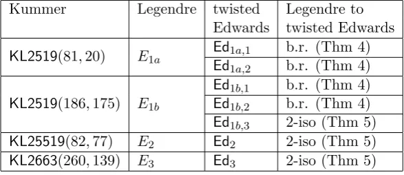
Table 7: Summary of the different twisted Edwards form curve. Here b.r. denotes birational equivalence and 2-iso denotes 2-isogeny.
Kummer Legendre twisted Legendre to Edwards twisted Edwards
KL2519(81,20) E1a
Ed1a,1 b.r. (Thm 4)
Ed1a,2 b.r. (Thm 4)
KL2519(186,175) E1b
Ed1b,1 b.r. (Thm 4)
Ed1b,2 b.r. (Thm 4)
Ed1b,3 2-iso (Thm 5)
KL25519(82,77) E2 Ed2 2-iso (Thm 5)
KL2663(260,139) E3 Ed3 2-iso (Thm 5)
3. Consider the applicability of Theorem 5. In this case, p ≡ 1 mod 4. So, the second case of Theorem 5 applies. This leads to the curve
Ed2 = EE,−1,d (60)
whered=−µ=a4/(b4−a4) =−6724/795.
The base point onEd2 corresponding to the point (x, y) on E2 given in Table 5 is obtained by applying the
map in (40) to (x, y). Denoting this point by (u2, v2), we have
u2 = 36371294725875594464038427339112611977790947606630656895088786307685446351235,
v2 = 5420399502534428101319348066018990605174033199858809431979181873337905014267.
(61)
Case 3: EE,−1,d arising from E3 =EL,µ arising from KL2663(260,139).
1. The co-factor of E2(Fp) is 12 and so by Proposition 1, there is no point of order 4. So, Theorem 3 does not apply.
2. Consider the applicability of Theorem 4. None of the choices ofα∈ {−ω,1−ω, µ−ω}lead to any solution. So, Theorem 4 does not apply.
3. Consider the applicability of Theorem 5. In this case, p ≡ 1 mod 4. So, the second case of Theorem 5 applies. This leads to the curve
Ed3 = EE,−1,d (62)
whered=−µ=a4/(b4−a4) =−67600/48279.
The base point onEd3 corresponding to the point (x, y) onE3 given in Table 5 is obtained by applying the
map in (40) to (x, y). Denoting this point by (u3, v3), we have
u3 = 89190048062212416001842209083228187904290557078088114148577357395664093858562357,
v3 = 5472512279031313112941693322256757737311467582966889426603287662650909757752053. (63)
6
Scalar Multiplication on Legendre/twisted Edwards Form Curves
For the twisted Edwards curves which are obtained from Legendre curves using a birational equivalence, the hardness of the discrete logarithm problem is preserved. For these twisted Edwards curves, it is sufficient to work only on these curves without reference to the underlying Legendre curves. So, the scalar multiplication algorithms for twisted Edwards curve using extended twisted Edwards coordinates can be applied. From Table 7, the relevant curves are Ed1a,1, Ed1b,1, Ed1b,2, Ed1b,3, Ed2,1, Ed3,1. For the twisted Edwards curves which are
obtained from Legendre curves using a 2-isogeny, it is required to work over the Legendre curves.
Following [7] scalar multiplication on the corresponding Legendre curves can be performed in the following manner. Let Φ (resp. Φ) be the 2-isogeny (resp. the dual 2-isogeny) from the Legendre form curve to the twistedb
Edwards form curve (resp. from the twisted Edwards form curve to the Legendre form curve). Let q be the largest prime dividing the order of the group ofFp rational points of the Legendre form curve. Let Pbe a point on the Legendre form curve of orderq andnbe a scalar. Sinceqis a prime, 2 has a multiplicative inverse modulo q. Following [7], the scalar multiplication nPcan be done in the following manner: P= Φ(P); n=n/2 modq; Q=nP;Q=Φ(Q); returnb Q.
The above requires an application of Φ andΦ each and a scalar multiplication in the twisted Edwards formb
curve. The times required for computing Φ and Φ are negligible in comparison to the scalar multiplication.b
Instead of directly computing the scalar multiplication on the Legendre form curve, this procedure benefits from the fast scalar multiplication possible on the twisted Edwards form curve.
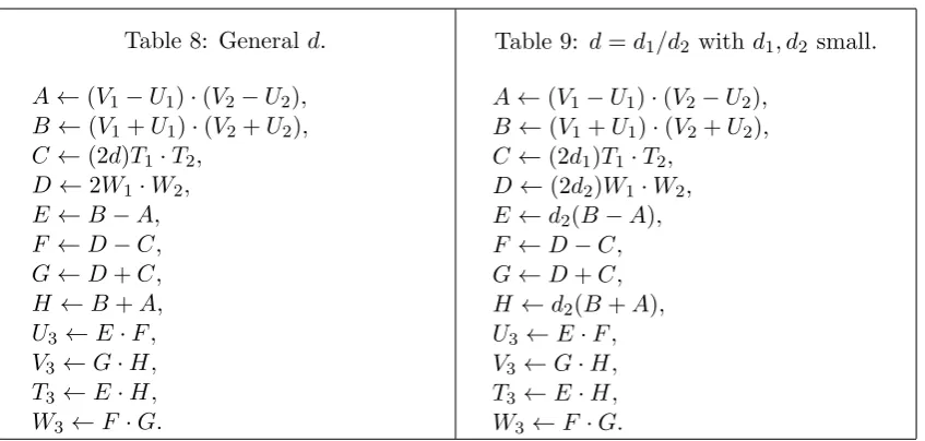
A unified addition algorithm using extended twisted Edwards coordinates for twisted Edwards curves of the form −u2 +v2 = 1 +du2v2 has been given in [13]. Suppose, it is required to add (U1 : V1 : T1 : W1),
(U2:V2 :T2:W2) and the result is (U3 :V3 :T3 :W3). The algorithm for performing this operation is shown in
Table 8. This requires a total of 8M+ 1C+ 8Awhere the C is the multiplication by 2d. For the cases, where d is a general element of Fp, essentially 9M+ 8A is required. On the other hand, suppose that d=d1/d2 where
d1 and d2 are small integers. The values ofdarising in the cases ofEd1b,4,Ed2,2 and Ed3,2 can be written in this
form. In this case, the above computation for obtaining (U3 :V3 :T3 :W3) can be rewritten as shown in Table 9.
This requires 8M+ 4C+ 8A. In this case, the multiplications counted byC are indeed multiplications by small constants. In other words, instead of 9M+ 8A, the cost becomes 8M+ 4C+ 8A. This is advantageous only if the time required for four multiplications by small constants is lesser than a general field multiplication.
For fixed base scalar multiplication, the efficiency can be further improved as suggested in [6]. Suppose (U1 : V1 : T1 : W1) is the fixed base where W1 = 1 and T1 = U1V1. If the fixed base point is represented as
(U1−V1, U1+V1,2dT1) then in the computation in Figure 8, the following simplifications become possible. The
multiplication (2d)T1·T2 becomes (2dT1)·T2; the multiplication 2W1·W2 becomes 2W2; and the computations
U1−V1 and U1+V1 are not required. So, the overall cost becomes 7M+ 6A. It had already been pointed out
in [13] that usingW1 = 1 leads to a cost of 7M+ 1C+ 8A. UsingW1 = 1 in conjunction with the idea in [6] of
using (U1−V1, U1+V1,2dT1) representation of the fixed base point leads to the cost of 7M+ 6A.
7
Conclusion
Table 8: Generald.
A←(V1−U1)·(V2−U2),
B ←(V1+U1)·(V2+U2),
C ←(2d)T1·T2,
D←2W1·W2,
E ←B−A, F ←D−C, G←D+C, H ←B+A, U3 ←E·F,
V3←G·H,
T3←E·H,
W3←F ·G.
Table 9: d=d1/d2 withd1, d2 small.
A←(V1−U1)·(V2−U2),
B ←(V1+U1)·(V2+U2),
C←(2d1)T1·T2,
D←(2d2)W1·W2,
E ←d2(B−A),
F ←D−C, G←D+C, H ←d2(B+A),
U3 ←E·F,
V3←G·H,
T3←E·H,
W3←F ·G.
References
[1] J. Barwise and P. Eklof. Lefschetz’s principle. Journal of Algebra, 13(4):554–570, 1969.
[2] D. J. Bernstein. Curve25519: New Diffie-Hellman speed records. InPublic Key Cryptography - PKC, volume 3958 of Lecture Notes in Computer Science, pages 207–228. Springer, 2006.
[3] D. J. Bernstein and T. Lange. Explicit-formulas database. http://www.hyperelliptic.org/EFD/index. html, 2007.
[4] D. J. Bernstein and Lange T. Faster addition and doubling on elliptic curves. In Advances in Cryptology -ASIACRYPT, volume 4833 ofLecture Notes in Computer Science, pages 29–50. Springer, 2007.
[5] Daniel J. Bernstein, Peter Birkner, Marc Joye, Tanja Lange, and Christiane Peters. Twisted edwards curves. In Serge Vaudenay, editor,Progress in Cryptology - AFRICACRYPT 2008, First International Conference on Cryptology in Africa, Casablanca, Morocco, June 11-14, 2008. Proceedings, volume 5023 ofLecture Notes in Computer Science, pages 389–405. Springer, 2008.
[6] Daniel J. Bernstein, Niels Duif, Tanja Lange, Peter Schwabe, and Bo-Yin Yang. High-speed high-security signatures. J. Cryptographic Engineering, 2(2):77–89, 2012.
[7] Eric Brier and Marc Joye. Fast point multiplication on elliptic curves through isogenies. In Marc P. C. Fossorier, Tom Høholdt, and Alain Poli, editors,Applied Algebra, Algebraic Algorithms and Error-Correcting Codes, 15th International Symposium, AAECC-15, Toulouse, France, May 12-16, 2003, Proceedings, volume 2643 of Lecture Notes in Computer Science, pages 43–50. Springer, 2003.
[8] M. Prem Laxman Das and Palash Sarkar. Pairing computation on twisted edwards form elliptic curves. In Steven D. Galbraith and Kenneth G. Paterson, editors,Pairing-Based Cryptography - Pairing 2008, Second International Conference, Egham, UK, September 1-3, 2008. Proceedings, volume 5209 of Lecture Notes in Computer Science, pages 192–210. Springer, 2008.
[10] G. Frey and H.-G. R¨uck. The strong lefschetz principle in algebraic geometry. Manuscripta Mathematica, 55(3):385–401, 1986.
[11] P. Gaudry. Fast genus 2 arithmetic based on theta functions. J. Mathematical Cryptology, 1(3):243–265, 2007.
[12] P. Gaudry and D. Lubicz. The arithmetic of characteristic 2 Kummer surfaces and of elliptic Kummer lines. Finite Fields and Their Applications, 15(2):246–260, 2009.
[13] H¨useyin Hisil, Kenneth Koon-Ho Wong, Gary Carter, and Ed Dawson. Twisted Edwards curves revisited. In Josef Pieprzyk, editor, Advances in Cryptology - ASIACRYPT 2008, 14th International Conference on the Theory and Application of Cryptology and Information Security, Melbourne, Australia, December 7-11, 2008. Proceedings, volume 5350 ofLecture Notes in Computer Science, pages 326–343. Springer, 2008.
[14] Jun ichi Igusa. Theta functions. Springer, 1972.
[15] Sabyasachi Karati and Palash Sarkar. Kummer for genus one over prime order fields. In Tsuyoshi Takagi and Thomas Peyrin, editors,Advances in Cryptology - ASIACRYPT 2017 - 23rd International Conference on the Theory and Applications of Cryptology and Information Security, Hong Kong, China, December 3-7, 2017, Proceedings, Part II, volume 10625 ofLecture Notes in Computer Science, pages 3–32. Springer, 2017.
[16] Neal Koblitz. Elliptic curve cryptosystems. Math. Comp., 48(177):203–209, 1987.
[17] Victor S. Miller. Use of elliptic curves in cryptography. In Advances in Cryptology - CRYPTO’85, Santa Barbara, California, USA, August 18-22, 1985, Proceedings, pages 417–426. Springer Berlin Heidelberg, 1985.
[18] Peter L. Montgomery. Speeding the Pollard and elliptic curve methods of factorization. Mathematics of Computation, 48(177):243–264, 1987.
[19] D. Mumford. Tata lectures on theta I. Progress in Mathematics 28. Birkh ¨auser, 1983.
[20] Katsuyuki Okeya, Hiroyuki Kurumatani, and Kouichi Sakurai. Elliptic curves with the montgomery-form and their cryptographic applications. In Hideki Imai and Yuliang Zheng, editors,Public Key Cryptography, Third International Workshop on Practice and Theory in Public Key Cryptography, PKC 2000, Melbourne, Victoria, Australia, January 18-20, 2000, Proceedings, volume 1751 ofLecture Notes in Computer Science, pages 238–257. Springer, 2000.