Building an Efficient Lattice Gadget Toolkit: Subgaussian
Sampling and More
∗
Nicholas Genise
†Daniele Micciancio
‡Yuriy Polyakov
§March 12, 2019
Abstract
Many advanced lattice cryptography applications require efficient algorithms for inverting the so-called “gadget” matrices, which are used to formally describe a digit decomposition problem that pro-duces an output with specific (statistical) properties. The common gadget inversion problems are the classical (often binary) digit decomposition, subgaussian decomposition, Learning with Errors (LWE) de-coding, and discrete Gaussian sampling. In this work, we build and implement an efficient lattice gadget toolkit that provides a general treatment of gadget matrices and algorithms for their inversion/sampling. The main contribution of our work is a set of new gadget matrices and algorithms for efficient subgaus-sian sampling that have a number of major theoretical and practical advantages over previously known algorithms. Another contribution deals with efficient algorithms for LWE decoding and discrete Gaussian sampling in the Residue Number System (RNS) representation.
We implement the gadget toolkit in PALISADE and evaluate the performance of our algorithms both in terms of runtime and noise growth. We illustrate the improvements due to our algorithms by imple-menting a concrete complex application, key-policy attribute-based encryption (KP-ABE), which was previously considered impractical for CPU systems (except for a very small number of attributes). Our runtime improvements for the main bottleneck operation based on subgaussian sampling range from 18x (for 2 attributes) to 289x (for 16 attributes; the maximum number supported by a previous implementa-tion). Our results are applicable to a wide range of other advanced applications in lattice cryptography, such as GSW-based homomorphic encryption schemes, leveled fully homomorphic signatures, other forms of ABE, some program obfuscation constructions, and more.
1
Introduction
Many advanced applications of lattice cryptography require the generation of a random integer matrix
A ∈ Zn×m
q (with uniform entries modulo q) together with a strong trapdoor (typically a short∗ basis S for the lattice defined byA as a parity check matrix). The strong trapdoor is used to efficiently “invert” the classical Short Integer Solution (SIS) and Learning with Errors (LWE) functions fA(x) = Ax and gA(s,e) = stA+et associated to the matrix A. Theoretical solutions to these trapdoor generation and
function inversion problems have long been known [1, 6, 7, 33, 25]. However, the trapdoor constructions of [1, 6] and generic inversion algorithms of [7, 33, 25] are rather complex, inefficient, and not suitable for practice.
An important step towards bringing advanced lattice-based cryptographic applications to practice was taken in [37], where a new notion of trapdoor (and associated generation algorithm) is proposed. The
∗This work was sponsored by the Defense Advanced Research Projects Agency (DARPA) and the Army Research Laboratory (ARL) under Contract Numbers W911NF-15-C-0226 and W911NF-15-C-0233. The views expressed are those of the authors and do not necessarily reflect the official policy or position of the Department of Defense or the U.S. Government.
†[email protected], UCSD. ‡[email protected], UCSD. §[email protected], NJIT.
trapdoor of [37] transforms the problem of inverting the random functionsfA, gAto the problem of inverting
the same type of functionsfG, gG, but for a specific, carefully designed “gadget” matrixG, which admits
much simpler and faster inversion algorithms. Gadget matrices similar to the one of [37] had already been used in a number of previous works, starting from Ajtai’s first construction of “solved instances of the shortest basis problem” [1], and including virtually all works on (fully) homomorphic encryption schemes based on the LWE problem (e.g., see [12, 26]); though different works use the gadget matrix for somehow different purposes. In fact, there are several inversion problems associated to the gadget matrixG:
• Digit Decomposition: This is the problem of expressing an arbitrary vectoru∈Znq as a short vector
x such thatGx=u (mod q). This is perhaps the most basic use of the gadget matrixG, and plays an important role in the key-switching and multiplication operations of fully homomorphic encryption (FHE) schemes. For example, the binary decomposition gadget matrix G= [I,2I, . . . ,2k−1I] allows
to write any vector with entries inZq as a combinationPi2 ix
i of vectorsxi∈ {0,1}n with the{0,1} coefficients corresponding to the binary digits of the entries in u.
• Subgaussian Decomposition: This is a type of randomized digit decomposition, where a short vector x satisfying Gx = u (mod q) is chosen according to a distribution with desirable statistical properties. This alternative to the standard binary decomposition was suggested in [5] as a method to improve the noise growth in homomorphic computations using variants of the GSW homomorphic encryption scheme [26], and is potentially applicable to the key-switching and homomorphic multipli-cation operations of many other FHE schemes.
• LWE Decoding: GivenstG+etfor a sufficiently small error vectore, recover bothsande. This is the (deterministic) inversion problem for the standard (injective) LWE functiongG, which is used, for
example, in the decryption algorithms of LWE-based cryptosystems.
• Discrete Gaussian Sampling: Produce a sample from a discrete Gaussian distribution over the set of all integer vectors x such that fG(x) = u. This problem was the main focus of [37], and is
used, for example, in hash-and-sign lattice-based signatures and trapdoor delegation for identity-based encryption, among many other applications.
Very efficient gadget inversion algorithms were given in [37], but only for the Discrete Gaussian Sampling and LWE Decoding problems, and in the very special setting where the modulus q=bk is the power of a small base b. For the case of Discrete Gaussian Sampling, an equally efficient, but more general solution, was recently proposed in [23] for arbitrary modulusq, expanding the range of advanced lattice cryptography applications that admit a reasonably practical implementation. (E.g., see [19, 17, 30, 9, 29].) We remark that trapdoor inversion is the most complex operation in many applications of lattice cryptography, and effective solutions to gadget inversion play a critical role in determining the efficiency, quality and other performance characteristics of higher-level algorithms and the final applications.
The main focus of our work is Subgaussian Decomposition, a problem that has received little or no atten-tion so far, and still has the potential to substantially improve the efficiency of many important applicaatten-tions. The importance of subgaussian sampling is easily explained by comparing it to the related problems of Digit Decomposition and Discrete Gaussian Sampling. We recall that lattice-based cryptography directly supports linear homomorphic operations, but ciphertexts are noisy, and their quality degrades when performing ho-momorphic operations: the noise of a sumc0+c1 is the sum of the noise in the original ciphertexts c0, c1. More critically, when multiplying a ciphertext by a constantα, the noise scales by a factorα, which can be arbitrarily large. So, one needs to limit linear combinations to use only small coefficients. This is typically done using binary digit decomposition: given encryptionsciof 2im(fori= 0, . . . , k−1), one can compute an encryption ofαm(for a largeα <2k) by taking a 0−1 combinationP
iαici, whereα=Pi2 iα
noise growth is improved by a factor√nk. At the other end of the spectrum, pythagorean growth can also be achieved using Discrete Gaussian Sampling, as gaussian distributions are by definition also subgaussians. However, gaussian sampling is considerably more costly than digit decomposition, both in terms of running time, randomness and output quality: even with the improved algorithms of [23, 37], Discrete Gaussian Sampling is much more complex than a simple digit decomposition, and it necessarily produces “digits” (i.e., coefficients) that are larger than naive binary decomposition roughly by a factor Ω(√logk). The added algorithmic complexity and noise overhead make gaussian sampling unattractive in practice, and, perhaps not surprisingly, all implementations we are aware of use digit decomposition whenever possible.
Subgaussian decomposition has the potential to offer the best of both worlds: pythagorean additivity, but without the Ω(√logk) noise overhead of a full-blown discrete gaussian sampler. These potential advantages were already outlined in [5], but they were so far considered only of theoretical interest. In fact, none of the subsequent improvements and implementations [21, 15, 16, 39] make use of subgaussian sampling.
Our contribution The main contribution of our work is a set of new gadget matrices and algorithms for efficient subgaussian sampling. The improvements are not just theoretical/asymptotical, but very practical, as demonstrated by a concrete complex application: an implementation of a Key-Policy Attribute-Based Encryption (KP-ABE) scheme that speeds up previous implementation efforts by more than one order of magnitude. (See below and Sections 7 and 8 for details.) On the theoretical side, our algorithms and gadgets result in pythagorean error growth and optimal (essentially linear) time complexity. In practice, the algorithms are easy to implement and have very small hidden constants both in the number of operations they perform and the subgaussian parameters, offering a very attractive alternative to the naive deterministic digit decomposition methods currently used in the implementation of FHE and other related pritimives. Moreover, our gadgets and algorithms have a number of other useful properties that make them even more attractive in practice:
• All our algorithms require very little storage and only a modest (essentially optimal) amount of ran-domness. In particular, our gadget matrices have a very regular structure, and do not need to be explicitly stored.
• We support an arbitrary modulusq. This is not just of theoretical interest, as fast implementations of lattice cryptography [34, 36, 8, 32] require moduli of special form in order to make use of the Number Theoretic Transform (NTT).
• Our gadgets and algorithms support the “Full RNS” and “double CRT” techniques used to implement lattice cryptography with large modulus without the need for arbitrary-precision arithmetic libraries [24, 8, 32].
Beside subgaussian decomposition, we also provide very efficient algorithms for LWE Decoding and Discrete Gaussian Sampling that improve previous work [37, 23] by supporting arbitrary moduli and Full RNS implementations. (For Discrete Gaussian Sampling, algorithms supporting arbitrary moduli were already provided in [23], but for gadget matrices that do not support Full RNS implementations.)
Taken together, our algorithms provide a complete lattice gadget toolkit, offering efficient solutions to the full range of inversion problems encountered in lattice cryptography: Subgaussian Decomposition, LWE Decoding, and Discrete Gaussian Sampling. Our results are not just of theoretical interest, but are also relevant to the implementation and use of advanced lattice cryptography applications.
implementation (for a comparable level of security) by a factor ranging from 18x to 289x as the number of policy attributes grows from 2 to 16. For higher numbers of attributes, previous CPU implementations were not feasible (only a GPU implementation is known), while we were able to run our implementation within reasonable running times for as many as 128 attributes. Other operations are also faster in our implementa-tion, and memory requirements are also much smaller (by more than a factor of 2x in the simplest case of 2 attributes, and more than one order of magnitude at 16 attributes.) In summary, our results show that using our toolkit gadget inversion is no longer the bottleneck in efficient implementations of lattice cryptography, and it can be profitably used to achieve better performance and scalability both in theory and practice.
While in this paper we focused on the algorithmic core of a general gadget toolkit, and on a specific (but representative) application, our results are applicable to a wide range of other advanced applications in lattice cryptography. These include the use of subgaussian decomposition in GSW-based homomorphic encryption schemes [21, 16, 15], leveled fully homomorphic signatures [28], other forms of ABE [4], obfuscation of finite automata and branching programs using graph-induced encoding [31], and more.
Techniques Our efficient lattice gadget toolkit is based on better algorithmic solutions to known problems, but also on a new class of gadget matrices that enable our algorithmic improvements. While gadget matrices of the type used in [37] and our work are quite common in lattice cryptography, they have never been formally defined. In fact, as different applications and algorithms use the gadget matrices in somehow different ways, it was not even clear if one could meaningfully define gadget matrices as abstract mathematical objects, and most of previous works use the term “gadget” informally to identify specific constructions.
The starting point of our investigation is a simple, intuitive definition of gadget matrix, which turns out to be relevant to the solution of all algorithmic problems studied in this work. For any dimension n and modulus q(typically mandated by the application), a gadget of qualityβ is a matrixG∈Zn×w
q such that
any u∈ Znq can be represented as Gx=u for some small integer vector x∈ Zw of norm kxk ≤β. This definition is directly motivated by the Digit Decomposition problem, but as we show in Section 3, it is already enough to enable theoretically efficient solutions to all of the algorithmic problems discussed above. (See Theorem 3.1 and Corollary 3.1.) The generic solutions obtained from Corollary 3.1 are not suited for practice, both in terms of algorithmic complexity and output quality. Still, a generic definition of gadget is useful to delimit a design space which extends well beyond the simplest (and perhaps most natural) construction of decomposition gadget [1,2,22, . . . ,2k−1] corresponding to the the standard binary representation of a number as a sequence of bits. Other gadgets used in our work are digit decomposition gadgets [1, b, b2, . . . , bk−1] with a larger base b > 2, the CRT gadget [g1, . . . , gk] where gi = ((q/qi)−1modqi)·(q/qi) [11] (for composite moduli with relatively prime factorizationq=Q
iqi) as well as hybrids between the two approaches where eachgi is replaced by an appropriate multiple of a vector of the form [1, b, b2, . . . , bk−1].
encryption.
Related Work The first use of subgaussian decomposition appears in [5] in a theoretical form, not opti-mized for implementations. While the use of CRT gadgets for digit decomposition in the implementation of FHE schemes [8, 32] or even the foundation of Ring LWE [35] is not new, their applicability in the context of Gaussian or subgaussian sampling is, to the best of our knowledge, novel. Our CRT gadget algorithms can be seen as an extension of [37, 23, 11]. The CRT-like gadget proposed in [31] can be considered as a special case of ours whenbi=pi (assuming thatqi=pei), which implies the gagdet noise width is larger thanpi. In our CRT gadget,bis can be chosen independently from CRT moduliqi, enabling significantly more efficient implementations in the ring setting. Another related work is a deterministic, balanced digit decomposition for the “double CRT/RNS” gadget [24] in the “LoL” library [18, 40] (initially unknown to the authors).
In the ring setting, one method [20] to achieve better-than-generic, nlog2q, efficiency of “power-of-b” gadget discrete Gaussian sampling is to use the FFO style of discrete Gaussian samplers from [22] and [23, Section 4]. This incurs a logarithmic slowdown, logn, in time and space compared to using [23, Section 3] on the coefficients independently, which hasnlogqtime and space efficiency. Further, Section 6 of this work extends [23, Section 3] to the “double-CRT” setting [24], freeing implementations using discrete Gaussian gadget sampling from multi-precision numbers when the modulus is over 64 bits.
Organization The rest of the paper is organized as follows. In Section 2 we review some preliminary material. In Section 3 we present our general definition of gadget matrices. Next, in Section 4 and Section 5 we present our core gadgets and algorithms for subgaussian decomposition and LWE decoding with arbitrary modulus. In Section 6 we extend these algorithms to large composite moduli to allow efficient operations in CRT form without the need of multiprecision integer arithmetic. Section 7 and 8 we present our imple-mentation and experimental results. The generic subgaussian version of Babai’s nearest plane is described in the Appendix.
2
Preliminaries
We indicate numbers with lowercase letters, such as z ∈Z, vectors as bold lowercase letters,z∈ Zn, and matrices as uppercase bold letters, M ∈ Rn×n. The default norm used is the l2 norm of a vector unless
stated otherwise, though we will often use the max, orl∞, norm. For a real number r, denote drcas the
deterministic rounding function to a nearest integer ofr. Rounding a real vector is applied analogously, entry-wise. Many computations will be done over the integers modulo q, Zq. We view Zq through its balanced coset representatives in (−q/2, q/2] unless stated otherwise. For a positive integer baseband a non-negative integer u < bk, u’s b-ary decomposition is a vector [u]kb = (u0,· · ·, uk−1) ∈ {0,· · · , b−1}k and satisfies
P
ib iu
i=u. Whenb= 2, this is simplyu’s binary decomposition. Recall the Chinese Remainder Theorem for modular arithmetic. Let q be a positive integer with a prime factorization ofq =pe1
1 · · ·p
el
l =q1· · ·ql. Then by the Chinese Remainder Theorem (CRT), we have Zq ∼=Zq1× · · · ×Zql. The isomorphism φ(·) is given by φ(a) = (a modq1,· · ·, a modql) and its inverse isφ−1(a1,· · · , al) =Pi(ai)qi∗qˆi whereqi∗:=
q qi and ˆqi:= (qi∗)−1 modqi.
For a probability distributionχ, we denotee←χto meaneis sampled fromχ. Whenχ is trivial (often over a numberx), we will usee←xto be variable assignment as well. We will need the following, known as theGerˇsgorin Circle Theorem.
Theorem 2.1 (Gerˇsgorin) Let M be ann×n matrix with complex entries. For each rowi, let ri be the sum of its non-diagonal entries’ magnitudes: ri =Pj6=i|M(i, j)|. Then, the eigenvalues of M are all in
S
2.1
Subgaussian Random Variables
A random variableX overRissubgaussian[35, 42] with parameterα >0 if its (scaled) moment generating function satisfiesE[exp(2πtX)]≤exp(πα2t2) for all t∈
R. Scaling a subgaussian X by any c∈Rto c·X
yields a subgaussian random variable with parameter |c|α. If X is subgaussian with parameterα, then its tails are dominated by a Gaussian parameterized by α, Pr{|X| ≥ t} ≤ 2 exp(−πt2/α2). Any B-bounded
centered (E[X] = 0) random variable X is subgaussian with parameter B
√
2π. When X is subgaussian with parameter α and Y conditioned on X taking any value is subgaussian with parameter β, X +Y is subgaussian with parameter pα2+β2. This property is called Pythagorean additivity. The proof of the
following Lemma is derived by expandingE[exp(2πt(X+Y))].
Lemma 2.1 LetX, Y be discrete random variables over Rsuch thatX is subgaussian with parameterαand
Y conditioned on X taking any value is subgaussian with parameter β. Then, X +Y is subgaussian with parameterpα2+β2.
Proof: Expanding the moment generating function gives the result:
E[exp(2πt(X+Y))] =
X
z
X
χ
Pr{Y =z−χ|X =χ}Pr{X =χ}exp(2πtz)
=X
χ
Pr{X=χ}exp(2πtχ)E[exp(2πtY)|X=χ]
≤exp(πt2(α2+β2)).
A random vector xoverRn issubgaussian with parameterα >0 ifhx,uiis subgaussian with parameter
αfor all unit vectorsu. Using a similar calculation to the above, one can show that if each coefficient of a random vector is subgaussian with parameter αconditioned on the previous coefficients taking any values, then the vector is subgaussian with parameter α. The slightly more general fact below is needed for our algorithms. Its proof is analogous to the proof of Lemma 2.1.
Lemma 2.2 Let x be a discrete random vector over Rn such that each coordinate x
i is subgaussian with parameterαi given the previous coordinates take any values. Then,xis a subgaussian vector with parameter maxi{αi}.
Proof: As before, we expand the moment generating function:
E[exp(2πthx,ui)] =
X
χ
Pr{x= (χ1,· · · , χn)}exp(2πthχ,ui)
≤exp(πt2X
i
α2iu2i)
≤exp(πt2max i αi
2kuk2).
The jump to the inequalities skips the straightforward calculations (nearly the same calculations as in
Lemma 2.1).
We emphasize this fact, for without it one is left with an unnecessary √n term in the subgaussian parameter of subgaussian vectors. Now, that the sum of independently generated random vectors xand y
subgaussian with parametersαandβis a subgaussian vector with parameterpα2+β2immediately follows.
A main algorithm presented in this paper will rely on a linear transformation of a discrete subgaussian vector.
Lemma 2.3 (Simplified [35, Corollary 2.3]) Let x be a subgaussian random vector with parameter α
and letM be a linear transformation. Then,Mx is a subgaussian vector with parameter αλmax(MMT)1/2
2.2
Lattices
A lattice is a discrete subgroup ofRn. Equivalently, a lattice Λ can be represented as the set of all integer combinations of a basis B = [b1,· · · ,bk] ∈ Zn×k, Λ = {Pk
1zibi : zi ∈ Z} = L(B). Notice that any
permutation of basis vectors is another lattice basis. We only consider full-rank lattices (k=n). A lattice is an integer lattice if it is a sublattice of Zn. The dual lattice of Λ, denoted as Λ∗, is the set Λ∗ ={z∈ Rn:hz,Λi ⊆Z}. Given a basis Bfor Λ, its dual basis is B−twhich is also a basis for Λ∗. We will consider
direct sums of lattices, Λ = Λ1⊕ · · · ⊕Λland their dual lattices Λ∗ = Λ∗1⊕ · · · ⊕Λ∗l. The numberλi(Λ) is the radius of the smallest ball containingilinearly independent lattice vectors.
Given a basis B= [b1,· · · ,bn] for a lattice Λ, its Gram-Schmidt orthogonalization (GSO) is the set of vectorsBe = [be1,· · · ,ben] whereebiis the component ofbiorthogonal to span(b1,· · · ,bi−1). The GSO is not
another basis for the lattice in general, but it gives us a tiling ofRngiven by
Rn=∪x∈Λ(x+P1/2(Be)) where
P1/2(Be) :=Be ·(−1/2,1/2]n. Note that the GSO depends on the order of the vectors given. We define the
reverse order GSO analogously. The algorithms presented in this paper will all be instantiations of Babai’s greedy decoding algorithm known as thenearest plane algorithm [7].
Theorem 2.2 There is an algorithm which givenB,Be,t∈Rnreturns the unique lattice point int+P1/2(B∗)
in timeO(n2)and memoryO(n3)†.
Discrete Gaussians LetA⊂Rn be a discrete set, and let the (spherical) Gaussian function with widths
and centerc∈Rnbeρs,c(x) = exp(−πkx−ck2/s2). Letρs,c(A) =Py∈Aρs,c(y). The smoothing parameter
of a lattice [38] for some ε > 0, is dentoted as ηε(Λ), and it is defined as the minimum s > 0 such that
ρ(s·Λ∗)≤1 +. Whens= 1 andc=0, we denote this asρ(·). Then, the discrete Gaussian distribution has probabilityρs,c(x)/ρs,c(A) for eachx∈A. This distribution is denoted asDA,s,c. Polynomial time discrete
Gausisan sampling algorithms for general lattices and their cosets, with width above the GSO length of the input basis (times a small factor,ω(√logn) orO(√logn)), are given in [25, 13].
q-ary Lattices Throughout this paper we will mostly be concerned with q-ary lattices. These are full-rank integer lattices with q·Zk as a sublattice. Fix an integer q > 0 to be used as a modulus and let
m > w > n. A matrixA∈Zn×m
q isprimitive ifAZmq =Znq. Given anA∈Znq×m, we define the following lattices: Λ⊥q(A) = {z ∈ Zm : Az = 0 modq}, and Λq(A) = {v ∈
Zm : ∃ s ∈ Zn, vt = stA modq}.
These lattices satisfy the following duality relation: Λ⊥q(A)∗ =q·Λq(A). Further, the cosets of Λ⊥q(A), Λ⊥u(A) :={z∈Zm:Az=u modq}, are in bijection withZnq whenAis primitive. LetGbe an arbitrary, primitive matrix overZq. The following sampling problem, defined on the integer cosets of Λ⊥q(G), is needed for many advanced lattice crypto-schemes.
Definition 2.1 For a primitiveG∈Znq×w, the subgaussian decomposition problem with parameterαforG is to sample vectors x∈Zw subgaussian with parameter αsuch that u=Gx modq for arbitrary ugiven
as input.
Another name for this problem is subgaussian sampling. A generic adaptation of Babai’s algorithm (analyzed in the Appendix, called the subgaussian nearest plane algorithm) is used in [5] (AP14) to achieve subgaussian decomposition for a specificG. In general, this generic algorithm runs in timeO(k2), and uses spaceO(k3).
Another, related problem is the discrete Gaussian sampling problem.
Definition 2.2 For a primitive G∈Zn×w
q , the discrete Gaussian sampling problem with width s forGis to sample vectorsx∈Zw distributed asDZw,s conditioned onGx modq=ufor arbitraryugiven as input.
Efficient solutions with small s for commonly usedG’s are given in [37, 23]. Both of the above sampling problems have polynomial time solutions using randomized versions of Babai’s algorithm. In addition, we will consider decoding theq-ary code defined byGfor an arbitrary, primitive G.
Definition 2.3 For a primitiveG∈Znq×w, the LWE decoding problem with toleranceδ onGis to returns givenstG+et modq for an errorkek∞< δ.
Specifically, we want to efficiently decode G while maximizing δ ∈ [0, q/2). An efficient LWE decoding algorithm for a specific, commonly usedG(b= 2 in the paragraph below) with toleranceq/4 is provided in [37].
AGcommonly used in lattice crypto-schemes is defined as follows. Fix an integerb∈(1, q), known as the base, and letk=dlogbqe. The block-diagonal gadget matrix isG=In⊗gtwith blocksgt:= (1, b,· · ·, bk−1). A common basis for Λ⊥q (gt) [23]Sqhas a sparse, triangular factorizationSq =SD[23] (restated in Section 4.2 in this paper).
3
Gadget Matrices
In order to guide our search for gadget matrices with efficient inversion and sampling algorithms, we give a simple general definition of gadget. The definition is modeled after the properties required by the digit decomposition problem, perhaps the simplest and most natural application of gadgets. But, as we will see, this simple characterization is enough to guarantee (theoretical) solutions to all problems that arise in the application of gadgets in lattice cryptography.
Definition 3.1 For any finite additive groupA, anA-gadget of sizewand qualityβis a vectorg∈Awsuch that any group elementu∈Acan be written as an integer combinationu=P
igi·xi wherex= (x1, . . . , xw) has norm at mostkxk ≤β.
We are primarily interested in gadgets for A=Znq, in which case the gadget is conveniently represented as a matrixG∈Znq×wsuch that for anyu∈Znq there is a vectorx∈Zwof lengthkxk ≤βsuch thatGx=u (modq). We defined gadgets in terms of abstract groups to emphasize that the dimensionnand modulus
qshould be thought of as part of the problem specification (typically mandated by the target application), while thewandβ describe the size and quality of the solution. In particular, for any givennandq, one may consider multiple gadgets achieving different values ofwand β. Naturally, smallerwand β are preferable, but as we will see there is a natural tradeoff between these two values, and one may increaseβ in order to reducewand vice versa.
Before establishing a formal connection between the above definition and the notion of gadget informally defined in previous work, we make some important observations.
• The matrixGis necessarily primitive, i.e.,GZw
q =Znq. Moreover, any primitive matrix is aZnq-gadget for a sufficiently largeβ= maxumin{kxk:Gx=u (modq)}.
• If g ∈ Zk is a Zq-gadget of quality β, then G= I⊗gt ∈ Znq×w is a Z n
q-gadget of size w = kn and quality √nβ.
• All definitions and constructions are easily adapted to ideal lattices (as used in the Ring-SIS and Ring-LWE problems) simply by considering “structured gadgets” of the form G⊗[α1, . . . , αn] where [α1, . . . , αn] is an appropriateZ-basis of the underlying ring.
Based on the above observations, constructions may focus on the casen= 1, i.e., gadget vectorsg∈Zwq, and then extend the solution to largern(and possibly to the ring setting) using general techniques. In fact, this is how larger gadgets are built in all applications we are aware of. However, all the results in this section hold for arbitrary matrices, not necessarily with this tensor structure. So, for the sake of generality, we use matrix notation.
In order to justify our abstract definition of gadget, we show that it guarantees all other properties of gadgets used by lattice cryptography: it maps the gaussian distribution to an almost uniform vector
GDw
with respect toG. All these properties are proved by bounding the relevant parameters of the lattice Λ⊥q(G) defined byG.
Theorem 3.1 For any gadget matrix G ∈Znq×w of quality β, the lattice L = Λ⊥q(G) has a basis S with orthogonalized length kS˜k ≤ 2β +√w, successive minima λ1(L), . . . , λw(L) ≤ 2β +
√
w and smoothing parameterη(L)≤(2β+√w)ω(√logn).
Proof: We first bound the covering radiusµ(L). Letx∈Rwbe arbitrary, and lety=bxebe a nearest point inZw tox. There exists some integer vectorzof norm at mostβ such thatGz=−Gy modq. Therefore, the vectory+zis in Λ⊥q(G) and is at distance at mostβ+√w/2 fromxby two applications of the triangle inequality.
The other bounds immediately follow from general relations (satisfied by any lattice)λw(L)≤2µ(L) and
η(L)≤λn(L)ω( √
logn). Finally, any lattice has a basis with orthogonalized lengthkS˜k ≤λw(L).
Note, the proof and theorem easily generalizes to any finite abelian group. Using the bound on the smoothing parameter, and the short (orthogonalized) basis S ∈ Zw×w, we immediately get the following
applications. (E.g., for the subgaussian decomposition algorithm see the Appendix.)
Corollary 3.1 For any gadget matrixG∈Zqn×w of quality β ands≥(2β+ √
w)pω(logn), the distribu-tion GDw
Z,s is statistically close to the uniform distribution over Z n
q. Moreover, there are polynomial-time algorithms for the following problems:
• Discrete Gaussian Sampling for the function fG(x) = Gx (mod q) and input distribution DwZ,s with
s≥(2β+√w)pω(logn).
• Subgaussian Decomposition w.r.t Gwith parameters≥(2β+√w)·√2π.
• LWE decoding of gG(s,e)for any s∈Znq and kek∞≤q/2·(2β+
√
w).
We remark that the general solutions provided by this corollary are of theoretical interest, and not suitable for practice. They are provided here only as a general feasibility result, in order to identify classes of good gadget matrices. The rest of the paper is dedicated to showing that by carefully choosing the gadget vectorg, one can obtain constructions and algorithms that are not only theoretically efficient, but also easy to implement and extremely fast.
4
Subgaussian Gadget Decomposition
In this section we present our main algorithms for the problem ofsubgaussian gadget decomposition, defined in Section 2.2, using the gadget matrixG=In⊗gt. Since this decompositionG−1(u) = (g−1(ui))ni=1 can
be computed one component at a time (even in-parallel!) we restrict our attention to efficiently computing the subgaussian functiong−1:
Zq →Zk in the one-dimensional case, i.e., forn= 1.
The gadgets and algorithms in this section are parametrized by a “base” integerb, which we consider as fixed throughout the section, but can be used to achieve different efficiency/quality trade-offs. We distinguish two cases, depending on whether the modulus is a powerq=bk of the baseb, or an arbitrary integerq < bk. In either case, no assumption is made about the factorization of the modulusq. Later, in Section 6, we will extend the gadgets and algorithms from this section to provide optimized treatment of large moduli with useful co-prime factorizationq=Q
iqi, where the inputu∈Zq is given in CRT form (umodq1, . . . , umod
ql).
All algorithms in this section use the same gadget gt := (1, b,· · · , bk−1), for k = dlog
bqe, but with different subgaussian decomposition procedures depending on the whetherqis a power ofb. Notice thatgt is aZq-gadget of size kand qualityβ=
√
The main result of this section is summarized in the following theorem.‡
Theorem 4.1 For any integer baseb >1, integer modulusq >1,k=dlogbqeand gadgetgt= [1, b,· · · , bk−1], there is a subgaussian decomposition algorithmg−1 as follows:
• If q=bk, the algorithm runs in linear O(k) time (and space), uses log
2q random bits, and achieves
subgaussian parameter at most (b−1)√2π.
• If q6=bk, the algorithm runs in linear O(k)time (and space), uses at most klog
2q random bits, and
achieves subgaussian parameter at most (b+ 1)√2π,
Notice how the generic solution obtained by applying Theorem 3.1 to our gadgetgonly implies a polyno-mial time inversion algorithm with subgaussian parameter (b+1)·√2kπ, and quadraticO(k2) time complexity
(after a cubic timeO(k3) preprocessing). Depending on implementation details, this generic solution would also require the use of high precision floating point numbers§ and a substantial amount of randomness for high precision sampling. (For completeness, we provide a more detailed analysis of the generic solution in the Appendix.) By contrast, the solution described in Theorem 4.1 is much more efficient (linear time and space, with no need for preprocessing) and also achieves a smaller subgaussian parameter by a factor of√k. Moreover, our specialized algorithms use a relatively small (almost optimal) number of random bits, and can be implemented without the need for high-precision floating-point arithmetic.
A proof of Theorem 4.1 is given by the algorithms presented and analyzed in the next two subsections for the two separate casesq=bk andq < bk.
4.1
Power-of-Base Case
Here we consider the subgaussian decomposition problem for the gadget g= (1, b, . . . , bk−1) whenq=bk, and the input is given as a positive coset representativeu∈ {0,1,· · · , q−1}. Conceptually, our solution to this problem is just a specialized/optimized version of the randomized-rounding variant of Babai’s nearest plane algorithm [7, 5]. The general algorithm uses the Gram-Schmidt orthogonalization of a basis for the lattice Λ⊥q(gt) associated to the gadgetg. The optimization is based on the observation (from [37]) that for our gadgetgand modulusq=bk, the lattice Λ⊥
q(gt) has a very simple basisS, and an even simpler GSO ˜S:
S=
b
−1 . .. . .. b
−1 b
, Se=b·I.
Using this special structure, there is no need to explicitly compute and store the GSO, and the randomized-rounding nearest-plane algorithm can be implemented in linear time and spaceO(k). The specialized algo-rithm is best illustrated whenb = 2, in which case it computes a randomized “bit” decomposition ofu as follows:
1. Fori= 0,· · · , k−1:
(a) ifuis even, then setxi←0,
(b) ifuis odd, then choose xi← {−1,+1}uniformly at random
Updateu←(u−xi)/2.
‡This theorem is most relevant whenqis a relatively small modulus (sayq <264), so that arithmetic operations moduloq
can be performed with unit cost. For larger moduli, the theorem will be used as a building block for a more complex algorithm described in Section 6 using RNS/CRT representation for the elements ofZq.
Algorithm 1: g−1(u) forq=bk.
Input: u∈ {0,1,· · · , q−1}
Output: subgaussianx∈Λ⊥u(gt) with parameter (b−1)√2π
1 Letx←0
2 fori←0,· · ·, k−1 do
3 Lety←u modb∈ {0,· · · , b−1}.
4 if y= 0 then
5 xi←0.
6 else
7 with probability y/b, xi←y−b, andxi←y otherwise.
8 u←(u−xi)/b.
9 return x
2. Returnx= (x0, x1,· · ·, xk−1).
This is essentially the same as the standard (deterministic) bit decomposition algorithm, except that when the bit is 1, we use a random ±1 digit. Since ±1 have the same parity modulo 2, the algorithm works as expected, with the only difference that now each digit is a zero-mean random variable, and the final output is subgaussian with parameter√2π.
We can modify this algorithm to an arbitrary base b as follows. Let y := u modb ∈ {0,· · · , b−1} for an input u∈ Zq. Then, at each step, we pick the coset representative (of u with respect toZb) with expectation 0 from the set{y−b, y}. The resulting algorithm is given in Figure 1. One can verify that this is the subgaussian nearest plane algorithm (given in the Appendix) applied to the latticeL(S) = Λ⊥q(gt), so the correctness of the algorithm is straightforward. Efficiency is also easily analyzed by inspection. Notice that the algorithm is randomness efficient as it needs only one random number in Zb for every interation, for a total ofk·log2(b) = log2(q) random bits.
We remark that a similar algorithm is analyzed in [4], though with a loose bound on its subgaussian parameter (there is an unnecessary√kfactor in their subgaussian analysis). This section’s main contribution is how to generalize the algorithm to arbitrary modulusq, as described in the next subsection.
4.2
Arbitrary Modulus, Arbitrary Base
Unfortunately, the (randomized) nearest plane algorithm Λ⊥q(gt) does not specialize well when the modulus
q is not a power of b. The reason is that, while we can still use the same gadget g = (1, b, . . . , bk−1), the
corresponding lattice Λ⊥q(gt) has a slightly different basisS
q whose GSO is not diagonal, and not sparse. Our solution uses a technique developed in [23] for the discrete Gaussian sampling problem. Specifically, we use the fact thatSq admits a sparse, triangular factorization
Sq=
b q0
−1 . .. ... . .. b q
k−2
−1 qk−1
= b
−1 . .. . .. b
−1 b
1 d0
. .. ... 1 dk−2
dk−1
=SD (1)
where (q0,· · · , qk−1) are the (baseb) digits ofq, and the last column ofDis defined by the simple recurrence di=di−1b+qi with initial conditiond−1= 0. (Note thatbi+1di=q modbi+1∈ {0,· · · , bi+1−1}.)
Then, on inputu∈ {0,1,· · ·, q−1}, we proceed as follows:
1. Compute an arbitrary element u∈Zk of the lattice coset Λ⊥u(gt), for exampleu= (u,0, . . . ,0).
Algorithm 2: g−1(u)
Input: u∈ {0,1,· · · , q−1}
Output: subgaussianx∈Λ⊥u(gt) with parameter (b+ 1) √
2π 1 Letu←[u]kb,x,y←0
2 x←0,q= [q]kb.
3 set xk−1←0 with probability (q−u)/qandxk−1← −1 otherwise. 4 fori=k−2,· · ·,0 do
5 u←u−ui+1bi+1, q←q−qi+1bi+1.
6 Letc← −(u+xk−1q).
7 if c <0then
8 p←(c+bi+1),z← −1.
9 else
10 p←c, z←0.
11 setxi←z+ 1 with probabilityp/bi+1 andxi←z otherwise.
12 fori∈ {0,· · · , k−2} do
13 yi←b·xi−xi−1+xk−1·qi+ui.
14 yk−1← −xk−2+xk−1·qk−1+uk−1.
15 return y.
3. Pick a subgaussian sample from the lattice coset L(D) +t.
4. Apply the (sparse) linear transformationSto the sample, to obtain a subgaussian sample from Λ⊥u(gt).
Here the (randomized) nearest plane algorithm admits a simple and efficient specialization because it is applied to a basis,D, which has a diagonal GSO. The linear transformationsS−1andScan also be computed
in linear time because Sis sparse and triangular. As a result, the algorithm runs in linear time O(k) and does not require any pre-processing. Finally, we get an output with subgaussian parameter (b+ 1)√2πsince
Shas small spectral norm.
The actual algorithm is given in Algorithm 2. The algorithm directly implements the outline given above, but it is specialized/optimized to avoid the explicit computation of the sparse matricesS,D, and to use only integer numbers (avoids floating point numbers). Details about the correctness and analysis of the algorithm are provided in the rest of this section.
Lemma 4.1 The first loop of Algorithm 2 performs the subgaussian nearest plane algorithm (described gener-ically in the Appendix) on the lattice generated byD around targett:=−S−1[u]kb.
Proof: Let d be the last column of D. The last entry of t is tk−1 = −u/bk and the last entry of d is dk−1=q/bk. Therefore, we are randomly roundingxk−1 around the center
D
t,d˜E/kd˜k2=−u/q∈(−1,0].
For the remainder of the loop, we note thatt=−S−1·uhas entriest
i=−(P i
j=0uj·bj)/bi+1,represented by the recurrence relation ti = ti−1/b+ui/b, t0 = −u0/b. This matches the recurrence relation for d, di = (Pij=0qj·bj)/bi+1 sinced=S−1[q]kb, so we can compute the remaining centers for the nearest plane algorithm by these recurrences. Specifically, we are performing a randomized rounding around the centers
ci =ti−xk−1di =−(Pil=0ul·bl+xk−1·Pij=0qj·bj)/bi+1 ∈(−1,1).These centers are stored as c in the pseudocode. The variablezrepresents the two parallel planes (copies ofL([d1,· · · ,di−1]) shifted by integer
multiples ofdi) separated by ˜di. The lemma follows.
By storing d=S−1[q]kb in-advance, one can change the code to sample the firstk−1 coordinates of x
in-parallel sinceL(d0,· · · ,dk−2) =Zk−1⊕ {0}. The proof of Theorem 4.1 follows below.
Proof: For the caseq=bk, Algorithm 1 returns a subgaussian samplex∈Λ⊥u(gt) with parameter (b−1) √
2π
Alternatively, let q 6= bk. Now by Lemma 4.1, x after the first loop is so that Dx is the output of subgaussian nearest plane algorithm onDcentered around−S−1u. By Lemma 2.3,Sqx+uis a subgaussian vector with parameterpλmax(S·St)
√
2π, whereλmax(S·St) is the maximum eigenvalue ofS·St. A routine calculation forS·St’s entries and the Gerˇsgorin Circle Theorem (Theorem 2.1) implyλ
max(S·St)≤(b+ 1)2. Since during each iteration in the first loop we draw a random number inZbi to representp, the algorithm consumes exactly log2b(1 + 2 +· · ·+k) = log2b·(k2+k)/2 random bits.
5
Gadget Decoding
Here we discuss our main algorithm for the problem ofLWE gadget decoding, defined in Section 2.2, on the gadget matrix G=In⊗gt with entries in Zq, for an arbitrary modulusq. Given a vt=stG+et∈Znkq as input, we can break the vector intoncomponents of length k, then decode (in-parallel) each component with respect togt. Therefore, we focus on decodinggtas a gadget forZq.
Our algorithm and its respective gadgets are parameterized by an integer “base”b. We considerbas fixed in this section, though varyingb for a fixed modulusq yields efficiency/quality trade-offs for these gadgets. Later, in Section 6 we present a CRT gadget that can be used to efficiently decode an input given in CRT form.
Let k = dlogbqe and the gadget be gt = (1, b,· · · , bk−1). The vector gt is a size k gadget of quality (b/2)√k forZq. The results in this section are summarized in the following theorem.
Theorem 5.1 For every modulus q, and gadget gt= (1, b,· · ·, bk−1), there is a time and spaceO(k)
algo-rithm decoding gt with tolerance q/2(b+ 1).
A proof of Theorem 5.1 is given by the algorithm presented in this section. Note, Theorem 3.1 implies a polynomial time decoding algorithm for gt with error tolerance kek
∞ ≤ q/2
√
k(b+ 1). Our decoding algorithm is more efficient and has a higher error tolerance by a factor√kthan the general gadgets decoding guarantee given by Theorem 3.1.
An optimized, linear time and space O(k), decoding algorithm is given in [37] for the caseq=bk. The reason for this algorithm’s efficiency is that the commonly used basis for Λbk(gt) results in a linear time nearest plane algorithm. In more detail, a basis for Λbk(gt) in this case is the triangular matrixBbk=bk·S−t, whereSis the commonly used basis for Λ⊥bk(gt) presented in Section 2.2, and this basis has a GSO of (q/b)·I. However, the simple decoding idea presented in [37] fails whenq6=bk. Because Λq(gt)’s commonly used basis has a dense GSO, Babai’s nearest plane algorithm takes time O(k2) and space O(k3) when naively applied on Λ⊥q (gt).
Efficient Decoding Algorithm The intuition for our algorithm is best initially viewed through the case when q = bk. Given an input v, another way to decode the lattice Λ
bk(gt) is to use St as a linear transformation, decode Stv to the lattice bk ·
Zk with the nearest plane algorithm, then map the nearest
point in bk·
Zk back to Λbk(gt). This leads to a slightly stronger condition on the noise vectore since we now needSte∈ P
1/2(q·I), which is satisfied ifkek∞< q/2(b+ 1). Though there is no need to do this given
the algorithm in [37], this is essentially what we will do in the case whenq6=bk.
Overview The overview of our efficient decoding algorithm for an arbitrary modulus is as follows. First recall the sparse, triangular factorization of Λ⊥q (gt)’s commonly used basis given in section 2.2,S
q=SD. The duality relation for q-ary lattices, Λq(gt) =q·Λ⊥
q(gt)∗, dictates that a basis for Λq(gt) isq·Sq−t=S−t(q·D−t). Luckily, the matrix D−t is sparse with a diagonal GSO, and P
1/2(q·D˜−t)⊇ P1/2(q·I) (meaning we can
decode as long askek∞< q/2(b+ 1)). Therefore, we can decodegtby the following.
1. Given v, first applyStas a linear transformation.
Algorithm 3: DecodeG(v, b,r[q]k b)
Input: v∈Zk,b, andq= [q]k b.
Output: s∈Zq wherev=sgt+etas long as kek∞< q/2(b+ 1).
1 fori←0,· · ·, k−2 do
2 vi←bvi−vi+1.
3 vk−1←b·vk−1.
4 Letx←0and reg←0. 5 fori←0,· · ·, k−2 do
6 xi ← dvi/qcand reg←reg/b+bk−1·qi.
7 vk−1←vk−1+xi·reg.
8 xk−1← dvk−1/bkc.
9 Lets←xk−1 and reg←0. 10 fori←k−2,· · · ,0 do 11 reg←b·reg +qi+1.
12 s←s+xi·reg
13 returns modq.
Both steps can be computed in linear time and space, O(k), given the sparsity ofSandqD−t, and qD−t’s diagonal GSO.
The pseudocode for our algorithm is shown inDecodeG. In short, the algorithm has three components, where each is represented by a loop in the pseudocode. These components are to first compute the linear transformation on the input v←Stv, then to run the nearest plane algorithm on the lattice generated by
q·D−t, and finally to returnsrepresented as the first entry of the nearest lattice point in Λq(gt) moduloq. The proof of Theorem 5.1 follows from Lemmas 5.1 and 5.2 below.
Lemma 5.1 The second loop in DecodeG is an instantiation of Babai’s nearest plane algorithm on the latticeq·D−tgiven target Stv, running in time and spaceO(k).
Proof: Recall the structure of D from section 2.2, D= [M|d] where Mt = [Ik−1|0] and d has entries di = (q modbi+1)/bi+1, withq modbi+1 ∈ {0,1,· · · , bi+1−1}. Then, it follows thatqD−t has a similar
triangular, sparse structure. This is given byq·D−t=
qIk−1 0
ct bk
and the vector c∈Zk−1 has entries
ci =−bk−1−i·(q0+bq1+· · ·+biqi) = −bk−1−i·(q modbi+1)∈ [−q,0]. Further, the entries of csatisfy the recurrence relation −ci= −
(ci−1)
b +b k−1q
i with the initial condition−c0 =bk−1q0. The variable reg in
DecodeG storesci, and it is updated using the recurrence relation for c. The vectorxin the pseudocode stores the coefficients of the nearest lattice point expressed in the basis qD−t. The Lemma follows by
inspection.
Lemma 5.2 The last loop in DecodeGcomputess modqin time and space O(k).
Proof: Represent the first row ofB=S−tqD−t ash, and notehh,xi=s modq. A careful analysis of
qD−tandS−tgives us an expression forh’s entries: h
i=qi+1+bqi+2+· · ·+bk−i−2qk−1= q−(q modb
i+1)
bi+1 for
i∈ {0,1,· · · , k−2}andhk−1= 1. All but the last entry ofhsatisfy the recurrence relationhi=qi+1+b·hi+1
fori∈ {0,· · ·, k−2}, with an initial value ofqk−1 (which isnot the actual value ofh’s last entry). We use
this recurrence relation to computeh’s entries one at a time in the last loop, stored in the variable reg. The
6
Gadgets for the CRT Representation
Many applications of lattice gadgets require a large modulus that, for secure and functional sets of parameters, surpasses the native 64-bit integer arithmetic in a modern machine’s hardware. One common method to circumvent the use of multi-precision numbers is to pick a modulus of the form q=Qq
i with each qi less than 64 bits. Then, one can store an elementu∈Zq as itsChinese Remainder representation (CRT form¶) as (u modq1,· · ·, u modql) and perform computations via the Chinese Remainder Theorem, utilizing the ring isomorphismZq ∼=Zq1× · · · ×Zql. Simple forms of the gadget matrix (e.g. power of two matrix) are not compatible with this representation because the binary digits of a number cannot be easily recovered from the CRT components without a costly reconstruction phase involving large numbers moduloq.
In this section, we discuss a gadget for the CRT form. As usual, the gadget admits a compact (implicit) representation, and does not need to be computed and stored explicitly. Most importantly, the gadget allows us to use the algorithms in Sections 4 and 5 in order to perform subgaussian decomposition, discrete Gaussian sampling, and LWE gadget decoding all given input represented in CRT form. This has several theoretical and practical advantages: (1) the algorithms can be directly used by efficient applications that already store their numbers in CRT form, (2) our algorithms can be easily parallelized as they operate on each CRT component independently, (3) all algorithms only require arithmetic on small numbers (at most maxiqi) even if the modulusq=Qiqi may be very big. (Efficient solutions to Discrete Gaussian Sampling for the individual moduliqi, as needed by our CRT DGS algorithm, are given in [37, 23].) We remark that a balanced, deterministic digit decomposition is provided in [18, 40], and an LWE decoding algorithm for a CRT/RNS hybrid gadget for general rings is given in the library’s codek(without an analysis). Our results are summarized in the following theorem. We emphasize the analysis below assumes integer operations, including reductions moduloqi, are done in constant time. This is because our algorithms are best implemented when eachqi is less than 64 bits, avoiding the use of multi-precision numbers.
Theorem 6.1 Let q have factorizationq=Ql
i=1qi into coprime factors{qi},(bi)
l
i=1 be an l-tuple of bases
with bi < qi for all i, and let k=Pki where ki=dlogbiqie. There exists a gadget, g t
CRT, for Zq of size k and quality maxibi/2. Further, the gadget satisfies the following properties:
• Subgaussian decomposition can be performed in-parallel with l processors, each using time and space
O(ki), consuming less thankilog2qirandom bits ((log2(qi)random bits ifqi=bkii)) and with parameter at most (maxi(bi) + 1)
√ 2π.
• For any >0, discrete Gaussian sampling can be performed in-parallel withl processors, each in time and spaceO(ki)with widths≥O(b1.5
j )ηε(Zkj)for index j maximizing
p
2bj(bj+ 1)·ηε(Zkj).
• gt
CRT is decodable in-parallel withlprocessors in time and spaceO(ki)with toleranceq/(2 maxi(bi)+1).
As expected, each processor gets slightly more efficient wheneverqi=bkii. The algorithms are represented in Figure 1.
The CRT Gadget For each coprime factorqi, fix thebase-bigadget vector asgti := (1, bi,· · ·, bkii−1) where
ki=dlogbi(qi)e. Letk=
P
iki, qi∗ =q/qi, and ˆqi= (qi∗)−1 modqi. Consider the gadget vector, which we call thegeneral CRT gadget,gCRTt = (q1∗q1ˆ ·gt1,· · ·, ql∗qˆl·gtl) modq∈Z
1×k
q . This is a generalization of the gadgets (or implicit in algorithms) used in [11, 31, 32, 8]. As before, the gadget matrix is the block-diagonal matrixG:=In⊗gCRTt .Theorem 6.1 follows from the fact Λ⊥q(gtCRT) = Λ⊥q1(g
t
1)⊕· · ·⊕Λ⊥ql(g t
l),Theorem 4.1, and Proposition 3.1 in [23]. The parallel decoding algorithm is obtained by a slight adaptation toDecodeG presented in Section 5, and is analyzed in the Section 6.1. We prove the direct sum decomposition of Λ⊥
q(gtCRT) below.
Proof: For the inclusion ⊇, let xi ∈ Λ⊥qi(g t
i) be arbitrary with x = (x1,· · ·,xl) as their concatenation. Then, hxi,gtii=aqi ∈qi·Z andhx,gCRTi modq =P
l i=1q
∗
iqˆihxi,gii modq = 0 +· · ·+ 0 mod q. We
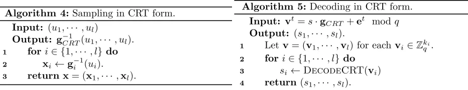
Algorithm 4: Sampling in CRT form.
Input: (u1,· · · , ul)
Output: gCRT−1 (u1,· · ·, ul).
1 fori∈ {1,· · · , l} do 2 xi←g−i1(ui). 3 return x= (x1,· · · ,xl).
Algorithm 5:Decoding in CRT form.
Input: vt=s·gCRT +et modq
Output: (s1,· · · , sl).
1 Letv= (v1,· · ·,vl) for eachvi∈Zki q .
2 fori∈ {1,· · ·, l} do
3 si←DecodeCRT(vi)
4 return(s1,· · ·, sl).
Figure 1: Pseudocode for the parallel algorithms given in Theorem 6.1. We let g−i1(·) denote either the subgaussian decomposition algorithm given in Section 4 or a discrete Gaussian sampler. The subroutine
DecodeCRTis a variation of the decoding algorithm given in Section 5 and is described in Section 6.1.
Algorithm 6: DecodeCRT(vi, bi,t= [qi]kbii, q, q∗i)
Input: vi∈Zki,bi,qi∗,q, andt= [qi] ki bi.
Output: s modqi wherev=sgt+et modqas long askek∞< q/2(bi+ 1).
1 forj←0,· · ·, ki−1do
2 vj ←bjvj−vj+1.
3 Letx←0.
4 forj∈ {0,· · · , ki−2}do
5 xj ← dvj/qc.
6 xk−1← d(vk−1−
c,xk0−2)/(qi∗biki)c.
7 Letsi←xk−1 and reg←0. 8 forj←ki−2,· · ·,0do 9 reg←b·reg +tj+1·q∗i.
10 si←si+xj·reg
11 returnsi modqi.
prove the converse by inducting on l, the number of q’s coprime factors. The base case is routine. Now considerx= (x1,· · · ,xl)∈Λq⊥(gtCRT) withxi∈Λ⊥qi(g
t
i) fori= 0,· · ·, l−1 andxl∈Zkl. By the inductive hypothesis,hx,gCRTi modq=ql∗qˆl·hxl,gtli= 0 modq.Viewing this equation inZand dividing both sides byq∗l implies ˆql· hxl,gli modql = 0.Finally, we conclude hxl,gli modql= 0 since ˆql is a multiplicative
unit inZql.
6.1
Decoding the CRT Gadget
Here we show how the efficient gadget decoding algorithm from Section 5 adapts to the general CRT gadget described in Section 6. Recall the decomposition ofgt’s lattice, Λ⊥q(gt) = Λ⊥q1(g
t
1)⊕ · · · ⊕Λ⊥ql(g t
l) =L(Sq1)⊕
· · · ⊕ L(Sql). The duality relation for q-ary lattices yields Λq(g
t) = q·(Λ⊥
q(gt))∗ = q·
L
iL(S− t qi D
−t qi)
= L
iL(S− t qiq
∗
i ·(qi·D−qit))
.
Now we have a clear way to decode the general CRT gadget. First, break the input into l blocks,
vt =sgt+et modq= (vt
1,· · ·,vtl) where v t
i =s·q∗iqˆigti+eti modq. Then, we compute the following. First, transform vi to Stqivi. Then, decode S
t
qivi to the latticeq
∗
i(qiD−qit). Finally, returns modqi. The pseudocode is given as the algorithmDecodeCRT. Another change is that we store the vectorcin memory. Recall,chask−2 entries of the formcj=−biki−1−j(qi modbji). Note that the correctness condition of our algorithm is stillketk
Decoding in CRT Form Here we describe how DecodeCRTcan decode v =sg+ewhere the input is given in its CRT representation. The ideas sketched here follow from [32]. The linear transformation
v → Stv is easily computed given the CRT form of v. Really, we are only concerned with divisions and integer rounding. In the second loop, note that xj ← dvj/qc = dP
l
o=1[(v modqo)·( ˆqo/qo)]c. Next we consider the line xk−1 ← d(vk−1+c,xk0−2
)/(q∗ibiki)c. First, note that vk−1/(bkiiqi∗) =b
−ki i ·
Pl
o=1(vk−1
modqo)·qˆo(qi/qo). This should be a small number in nearly all practical instantiations. Lastly, we note that we returnsin CRT form, but we can alter the algorithm to returns∈(−q/2, q/2] via a simple change. Thescomputed in the last loop is actuallys·qi∗qˆi. So, we can remove the modqiin the return statement and sum up the output from thel parallel processors,P
i(s·qi∗qˆi) =s·
P
i(qi∗qˆi) =s·1 modq.
7
Toolkit Implementation and Its Application
7.1
Software Implementation
We implemented most of the algorithms presented in this work in PALISADE [41], a modular open-source lattice cryptography library that includes ring-based implementations of homomorphic encryption, proxy re-encryption, identity-based encryption, attribute-based encryption, and other lattice schemes. More con-cretely, we added a new lattice gadget toolkit module to PALISADE that implements the following algo-rithms:
• Subgaussian gadget decomposition (Algorithm 2) for arbitrary moduli and gadget bases.
• Efficient gadget in CRT representation, enabling both trapdoor sampling and subgaussian gadget decomposition in the CRT representation.
• Subgaussian gadget decomposition for cyclotomic rings both in positional and CRT number systems, which wraps around Algorithm 2.
The toolkit module complements/improves the lattice gadget algorithms previously added to PALISADE, such as trapdoor sampling for cyclotomic rings proposed in [23] and implemented in [30, 17]. The full lattice gadget capability will be included in the next major public release of PALISADE.
7.2
Optimized Variant of Key-Policy Attribute-Based Encryption
We use the lattice gadget toolkit algorithms to build and implement a full RNS/CRT variant of the short-secret Key-Policy Attribute-Based Encryption (KP-ABE) scheme originally proposed in [10] and imple-mented for cyclotomic rings in [19]. The KP-ABE scheme is a complex cryptographic primitive that can be used for attribute-based access control applications, as well as a building block for audit log encryption, targeted broadcast encryption, predicate encryption, functional encryption, and some forms of program obfuscation [10, 27].
7.2.1 Overview
ABE is a public key cryptography primitive that enables the decryption of a ciphertext by a user only if a specific access policy (defined over`attributes) is satisfied. In the key-policy scenario, a message is encrypted using the attribute values as public keys, and a specific access policy is typically defined afterwards. When the access policy becomes known, a secret key for the policy is generated (using trapdoor sampling in our KP-ABE scheme), and the ciphertexts and public keys are homomorphically evaluated over the policy circuit (using a GSW-type homomorphic multiplication in our KP-ABE scheme).
The short-secret KP-ABE scheme is a tuple of functions, namely Setup, Encrypt, EvalPK, KeyGen,
• Setup(1λ, `)→ {MPK,MSK}: Given a security parameter λand the number of attributes `, a trusted private key generator (PKG) generates a master public key MPK and a master secret key MSK. MPK
contains the ABE public parameters whileMSKincludes the trapdoor that is used by PKG to generate secret keys for access policies.
• Encrypt(µ,x,MPK)→C: Using MPKand attribute valuesx∈ {0,1}`, sender encrypts the messageµ and outputs the ciphertextC.
• EvalPK(MPK,x, f)→PKf: Homomorphically evaluateMPKover a policy (Boolean circuit)f :{0,1}`→ {0,1} to generate a public keyPKf for the policyf.
• KeyGen(MSK,MPK,PKf) → SKf: Given MSK, MPK and policy-specific PKf, PKG generates the secret key SKf corresponding tof. PKG sendsSKf to the receiver that is authorized to decrypt ciphertexts encrypted underf.
• EvalCT(C,x, f) →Cf: Homomorphically evaluate C over the policy f to generate the ciphertext
Cf.
• Decrypt(Cf,SKf) → µ¯: Given the homomorphically computed ciphertext Cf and corresponding
secret key SKf, find ¯µ, which is the same as the original messageµ if the receiver has the secret key matching the policyf.
The most computationally expensive operations are EvalPK and EvalCT, which homomorphically evaluate a circuit of depthdlog2`eusing the GSW homomorphic multiplication approach. At each level of a Boolean circuit composed of NAND gates (which are used for benchmark evaluation in [19]), the algorithms compute matrix productsB2iG−1(−Bi) and G−1(−Ci)
t
C2i for public keys and ciphertexts, respectively. Here, Bi ∈ R1q×m, Ci ∈ Rmq , Rq = Zq[x]/hxn+ 1i, and m = dlogbqe+ 2 (the latter corresponds to the Ring-LWE trapdoor construction). Note that that the gadget Gis extended in this case tom by adding two zero entries to the decomposed digits.
The work [19] presents a CPU implementation of the ring variant of the KP-ABE scheme along with an efficient GPU implementation for policy evaluation and encryption. The CPU implementation was done for a binary gadget base and used the conversion from CRT to the positional number system for digit decomposition both in trapdoor sampling and gadget decomposition. To avoid the linear noise growth
O(nm) in gadget decomposition, the authors used a balanced digit decomposition, namely the binary non-adjacent form (NAF), that replaces digits in (0,1) with a zero-centered representation in (-1,0,1). Although this approach allows one to achieve a heuristic growth close toO(√nm) in the case of the KP-ABE scheme, the noise properties depend on the randomness of the input, i.e., this approach is deterministic.
The CPU runtimes for policy evaluation and encryption operations in [19] were far from practical (the CPU results only for`up to 8 are presented), and hence the authors developed an efficient GPU implemen-tation for these operations.
For detailed algorithms of the KP-ABE scheme, the reader is referred to [19].
7.2.2 Our Optimizations
We present a full CRT/RNS ring variant of the KP-ABE scheme that leverages the lattice gadget toolkit to significantly (by more than one order of magnitude) speed up the policy evaluation operations. In particular, our implementation includes the following optimizations as compared to [19]:
0 5 10 15 20 25 30 0
2 4 6 8 10 12
b=2
r
arbitrary b
S
a
m
p
l
i
n
g
r
a
t
e
(
i
n
1
0
6
p
e
r
se
co
n
d
)
log
2
b
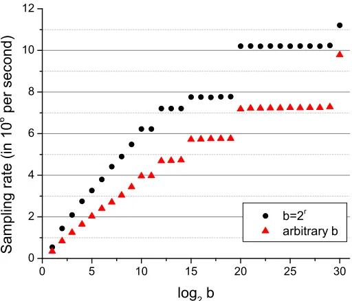
Figure 2: Runtime baseline of subgaussian sampling rate for native uniformly random integers (w.r.t a 60-bit modulus). When b= 2r, the modulo reduction in digit decomposition is performed by simple bit shifting. Whenb is arbitrary, the slower hardware modulo operation is used. The plateaus correspond to the same number of digits, i.e., the same value ofd60/log2be.
• The CRT variant of trapdoor sampling using the gadget decomposition technique discussed in this paper in contrast to the multiprecision digit decomposition in [19].
• The RNS/CRT scaling proposed in [32] for decryption in constrast to the multiprecision scaling.
• Increased gadget baseb(both in trapdoor and subgaussian gadget decomposition) instead of the binary base.
7.2.3 Parameter Selection
As the correctness constraint in [19] was derived for the classical binary-base gadget decomposition, we provide here a modified version incorporating the effect of a larger gadget base for the case of subgaussian gadget decomposition:
q >4C1sσ
√
mn b√mnd
, (2)
whereC1= 128,s=C·σ2(b+ 1)·(
p
nlogbq+√2n+ 4.7), C= 1.8,σ≈4.578, andd=dlog2`e. Here,C
andC1are empirical parameters chosen the same way as in [19].
0 100 200 300 400 500 600 1
10 100 1000
CRT (arbitrary b)
CRT (b=2
r
)
MP (arbitrary b)
MP (b=2
r
)
P
o
l
yn
o
m
i
a
l
sa
m
p
l
i
n
g
r
a
t
e
(
p
e
r
se
co
n
d
)
Bits in modulus
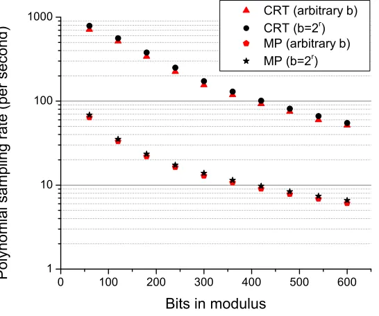
Figure 3: Comparison of sampling rates for CRT and multiprecision (MP) variants of subgaussian gadget decomposition for ring elements with 4096 coefficients and 60-bit CRT moduli at r =dlog2be= 20. The MP variant requires converting from CRT representation to positional number system followed by digit decomposition w.r.t. a large integer.
8
Experimental Results
We ran the experiments in PALISADE version 1.2, which includes NTL version 10.5.0 and GMP version 6.1.2. The evaluation environment was a commodity desktop computer system with an Intel Core i7-3770 CPU with 4 cores rated at 3.40GHz and 16GB of memory, running Linux CentOS 7. The compiler was g++ (GCC) 5.3.1.
8.1
Subgaussian Gadget Decomposition
The experiments described in this section were all performed in the single-threaded mode. The goal of these results is to provide the performance baselines for subgaussian gadget decomposition, demonstrate the benefits of the efficient gadget in CRT representation, and illiustrate the effect of subgaussian sampling on the noise growth in GSW-type products.
0 2 4 6 8 10 0
20 40 60 80 100 120 140 160
Subgaussian
Classical
N
o
i
se
l
e
ve
l
(
i
n
b
i
t
s)
Depth
Equation y = a + b*x
Value Standard Error Subgaussian
Intercept 3.65547 0.33142 Slope 8.70829 0.05341 Classical
Intercept -5.37852 0.63843 Slope 15.63138 0.10289
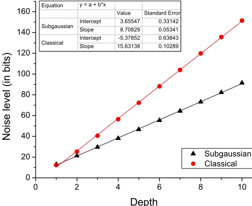
Figure 4: Noise growth for GSW-type multiplication in the ring-based KP-ABE variant (k= 180,n= 1024,
b = 2). The base in the exponentiation is (mn)β, where m = k+ 2 = 182 and β describes the rate of noise growth. The slope of the linear interpolation is βlog2(mn). The values of β are 0.497 and 0.893 for subgaussian and classical gadget decomposition, respectively.
efficient implemention of arithmetic over prime powers is available) over power-of-two bases.
Figure 3 illustrates the benefits of using the efficient gadget in CRT representation when working with cyclotomic rings. The conversion from CRT representation to the positional system followed by digit decom-position w.r.t a large modulus slows down subgaussian gadget decomdecom-position rate by almost one order of magnitude. We also observe that the difference in performance between a power-of-two base and an arbitrary base is relatively small for both cases.
Figure 4 demonstrates the differences in the noise growth of GSW-type products using the subgaussian and classical binary gadget decomposition methods. For this experiment, we generated an error vector inRm and iteratively multiplied it byG−1(U
i), whereUi is a vector of unformly random ring elements in Rmq at leveli. We applied the tree multiplication approach (rather than a sequential evaluation in a right-associative manner, which reduces the noise when dealing with a chained product of fresh encryptions in GSW [14, 5]) to emulate the noise growth in evaluating a Boolean policy circuit in the KP-ABE scheme. We considered both the cases when the sameUwas used at all levels (correlated ciphertexts) and differentUi at each level. The results were approximately the same for both scenarios because the classical gadget decomposition matrix is centered at 0.5 (see [19] for a more detailed discussion of the classical gadget decomposition case).
![Table 1: Comparison of performance results for our KP-ABE variant (in bold) vs.theimplementation in [19] (in parentheses)](https://thumb-us.123doks.com/thumbv2/123dok_us/7972507.1322057/22.612.72.546.126.230/table-comparison-performance-results-abe-variant-theimplementation-parentheses.webp)
