A feature extraction method based on VMD and RDT
and its application in engine crankshaft bearing fault
Gang Ren 1, Jide Jia 2, Jianmin Mei2, Xiangyu Jia 1, Jiajia Han 1
1 Postgraduate Training Brigade,Army Military Transportation University, Tianjin 300161, China;
[email protected] (G.R.); [email protected] (X.J.); [email protected] (J.H.)
2 Military Vehicle Department, Army Military Transportation University, Tianjin 300161, China;
[email protected] (J.J.); [email protected] (J.M.)
* Correspondence: [email protected] or [email protected] ; Tel:+86-022-84658841
Abstract. The vibration signal of the engine contains strong background noise and many kinds of modulating components, which is difficult to diagnose. Variational mode decomposition (VMD) is a recently introduced adaptive signal decomposition algorithm with a solid theoretical foundation and good noise robustness compared with empirical mode decomposition (EMD). VMD can effectively avoid endpoint effect and modal aliasing. However, VMD cannot effectively eliminate the random noise in the signal, so the random decrement
technique is introduced to solve the problem.Based on the crankshaft bearing fault simulation
experiment, the four kinds of wear state vibration signals are decomposed by VMD, and the
modal components with smaller permutation entropy are selected as fault components.Then
the fault component is processed by the random decrement technique, and the Hilbert
envelope spectrum of the fault component is obtained. Compared with the fault feature
extraction method based on EMD and EEMD, the feature extraction results of the proposed
method are better than those of the above two methods. The simulation analysis and the
simulation test of the crankshaft bearing fault verify the effectiveness of the proposed method.
Keywords: variational mode decomposition; random decrement technique; crankshaft bearing; engine; feature extraction
1 Introduction
The engine is a complex mechanical device, with the characteristics of multi-source, multi moving parts, and complex work. The engine has both rotational and reciprocating motion.
Vibration signals are fully used in fault diagnosis because of their convenience [1-2]. The
vibration signal of engine is composed of multi-component complex signals, and its amplitude varies with time. For the complex multi-component signal, it is usually necessary to decompose it into a number of single-component AM-FM signals, and each component is analyzed to extract amplitude and frequency information.
In order to solve the above problems, Huang et al. introduced an adaptive signal processing
technique called empirical mode decomposition (EMD) [3-4], which has demonstrated
outstanding performance in dealing with nonlinear and nonpstationary signals. This technique
has been applied in many fields, such as biomedical image analysis [5], fault diagnosis of rolling
element bearings [6], signal de-noising [7-9], and voice signal analysis [10]. But there are still
some problems for EMD, such as endpoint effect and modal aliasing [11]. Wu [12] proposed
Ensemble Empirical Mode Decomposition (EEMD). Different white noises are added to the
original signal for EMD, and multiple decomposition results are averaged to obtain the final Intrinsic Mode Function (IMF). The high frequency modulation information in the signal can be
separated very well, and the modal aliasing of EMD is well suppressed [13].However, the white
noise can easily lead to the reconstruction error for EEMD.
In recent years, Konstantin, Dragomiretskiy et al. proposed variational modal
decomposition [14], which is essentially composed of several adaptive Wiener filters and has
good noise robustness. Compared with EMD, VMD has strong mathematical theory basis. So it can effectively alleviate or avoid a series of problems that exist in EMD, and has higher
operation efficiency. VMD is widely used in various engineering fields [15-18]. An X.L. et al.
applied VMD to the bearing fault diagnosis of the wind turbine, and realized the effective
discrimination of the bearing fault [19]. By combining VMD with detrended fluctuation analysis
(DFA), Liu et al. successfully extracted gear fault characteristics [20]. By combining VMD with
independent component analysis (ICA), Yao et al. successfully separated the piston knock and
combustion noise of the engine [21]. However, there is nothing VMD can do about the random
noise in the signal.
In order to solve the problem, the random decrement technique (RDT) is introduced in this
paper. Random decrementtechnique is a method of identification of modal parameters, which
is first proposed by Cole [22-23] in 70s. The basic concept of RDT is to assume a system with
stationary random excitation, and its response is the superposition of both deterministic and
random responses.The deterministic response is separated from the random response, and
the random response is eliminated by using the statistical mean method. Finally, a
deterministic free attenuation signal is obtained by filtering.RDT has been widely used in many
fields such as vibration modal analysis [24], and structural damage detection [25].
In this paper, a new fault feature extraction method for engine crankshaft bearing is proposed based on the variational mode decomposition and random decrement technique. First, the VMD is used to decompose the fault signal into several modal components, and the
fault components are selected according to the permutation entropy. Then the fault
component is processed by the random decrement technique and the Hilbert envelope
spectrum is calculated to extract the fault features.The effectiveness of the proposed method
is verified by simulation analysis and the simulation experiment of crankshaft bearing fault.
2 Variational Mode Decomposition
The VMD algorithm defines the intrinsic mode function as a non-stationary AM-FM signal. The intrinsic mode is considered as follows:
))
(
cos(
)
(
)
(
t
A
t
φ
t
u
k=
k k (1)Where the phase
φ
k(
t
)
shall satisfy the following condition:φ
k(
t
)
′
≥
0
; the envelopeline
A
k(
t
)
should satisfy the following condition:A
k(
t
)
≥
0
; the instantaneous frequency)
(
t
ω
k should satisfy the following condition:ω
k(
t
)
=
φ
k(
t
)
′
.A
k(
t
)
andω
k(
t
)
changeslowly, and
φ
k(
t
)
changes more rapidly.The Hilbert transform is performed for each modal function
u
k(
t
)
, and exponentialcorrection is applied to obtain K modal functions. Then the frequency spectrum of the modal function is corrected to the estimated central frequency, and the bandwidth of the modal component is calculated by using Gauss smoothing. The variational constraint problem can be defined as follows:
}
)}
(
*
]
)
(
{[(
{
min
2
2 1
} { },
{
∑
K
k
t ω j k t
w u
k k
k
e
t
u
t
π
j
t
δ
a
=
+
∑
K
k
t
f
t
s
1
)
(
.
.
=
Where
u
k is the modal component,ω
k is the central frequency for the modalcomponent,
δ
(
t
)
is the unit pulse function, and * is the convolution symbol.In the VMD algorithm, the secondary penalty factor and the Lagrangian multiplication
operator are used. Then, the alternating direction method is introduced.
u
kn+1,ω
kn+1, and1 +
n
λ
are constantly updated, so that the optimal solution of the variational constraint problemcan be solved. The expression for the modal component
u
kn+1 is} 2 ) ( ) ( ) ( )} ( * ] ) ( {[( { 2 2 2 2 1
∑
argmin ∈ i i t ω j k t X u n k t λ t u t f e t u t π j t δ a α u k k + + + =+ (3)
where
α
is the penalty factor, andλ
is the Lagrange multiplier.The expression for the modal component
u
kn+1 in frequency domain is2 1
)
(
2
1
1
)
2
)
(
ˆ
)
(
ˆ
)
(
ˆ
(
)
(
ˆ
k i i n kω
ω
α
ω
λ
ω
u
ω
f
ω
u
-
∑
+
+
=
+
(4)
Where
ω
k is the center of the modal component power spectrum. The Wiener filter isintroduced, which makes the VMD algorithm have better noise robustness.
Similarly, the expression for the central frequency
ω
kn+1 isω
d
ω
u
ω
d
ω
u
ω
ω
ω
k k n k 2 0 2 0 1)
(
ˆ
)
(
ˆ
)
(
∫
∫
∞ ∞=
+ (5)The stopping condition of the iteration is
e
u
u
u
knK k n k n k
<
= + 2 2 2 2 1 1ˆ
/
ˆ
ˆ
∑
(6)According to the previous derivation, we get the complete algorithm for VMD, summarized in algorithm 1.
algorithm 1: Complete optimization of VMD Initialize
{
u
ˆ
1k}
,{
ω
ˆ
k1}
,{
λ
ˆ
1}
,n
←
0
repeat
1
+
n
n
←
for k = 1:K do
Update
u
ˆ
kn+1 for all w >=0:Update wk:
ω
d
ω
u
ω
d
ω
u
ω
ω
ω
k k n k 2 0 2 0 1)
(
ˆ
)
(
ˆ
)
(
∫
∫
∞ ∞←
+ (8) end forDual ascent for all w>=0:
] ) ( ˆ ) ( ˆ [ ) ( ˆ ) ( ˆ 1 1 1
∑
← K k n k n n ω u ω f β ω λ ω λ = + ++ (9)
until convergence:
e
u
u
u
knK k n k n k
<
= + 2 2 2 2 1 1ˆ
/
ˆ
ˆ
∑
(10)The VMD algorithm is a linear transformation, so the signal can be reconstructed. The reconstructed signal can be represented as:
∑
K k ku
t
f
1ˆ
)
(
ˆ
==
(11)Where
u
ˆ
k is the final modal component, after the iteration is stopped.3 Random Decrement Technique
RDT can be used to describe the impulse response of the system, and its advantage is that
it can extract free impact response from the stationary random response in the system. The
core is to assume that a system is subjected to stationary random excitation, and the response
is the superposition of deterministic responsedetermined by the initial condition and random
responsedetermined by the initial external load.Under the same initial conditions, stationary
random response is divided into several sections, and the general mean of the intercept segments is calculated, so as to extract the free attenuation response.
The response signal is divided into L segments, and each segment of the signal is
expressed as xi(t), whose length is .Each response signal has the same trigger value, and the
trigger value can be expressed as
L
i
const
x
t
x
i(
i)
=
s=
,
=
1
,
2
,
,
(12)The overall mean of the L segment signal is calculated, and the random decrement function can be expressed as:
)
(
Σ
1
)
(
1
x
t
τ
L
τ
x
i iL i
+
=
= (13)where
x
i(
t
i)
=
x
s,
i
=
1
,
2
,
,
L
.4 Proposed Method
fault characteristics from the vibration signals of engines.
The permutation entropy is a new method of mutation detection, which mainly aims at
the spatial characteristics of time series [26-27]. The permutation entropy is very simple in
theory and has good noise robustness. Besides, the permutation entropy also has a high resolution, and the output results are very intuitive. The permutation entropy reflects the random degree of the signal. In other words, the smaller the permutation entropy, the more
fault information the time series has.Therefore, the permutation entropy is used to select the
fault component in this paper.
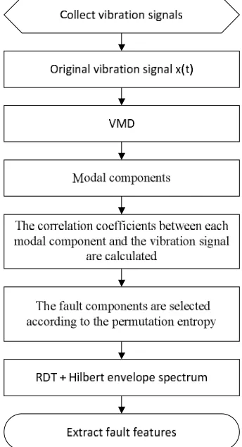
VMD is a recently proposed signal decomposition method, which is essentially composed of a number of adaptive Wiener filters, and has good noise robustness. Compared with the EMD method, the VMD method has a solid mathematical theoretical foundation, and can effectively alleviate or avoid a series of shortcomings in the EMD method. To verify the efficiency of the proposed method, several experiments on engine crankshaft bearing faults are performed. The detailed experimental scheme is shown in Figure 1. Firstly, a single channel vibration signal x(t), which is a wearing fault of the engine crankshaft bearing, is collected by the acceleration sensor vertically fixed on the engine block. Secondly, the collected vibration
signal x(t) is decomposed into several modal components by VMD method. Thirdly, the
permutation entropy of each modal component is calculated respectively, and the modal components with smaller permutation entropy are selected as the fault components. Lastly, the fault components are processed by the random decrement technique and the Hilbert envelope spectrum is calculated to extract the fault features.
5 Experimental Results 5.1 Simulation
Engine crankshaft bearing consists of two bearing bushings. When the crankshaft bearing has a wear fault, it is mainly under attack by the rotation of the crankshaft and the ignition of the cylinder. Therefore, the characteristic frequency of engine crankshaft bearing fault is mainly the rotation frequency of engine crankshaft and the ignition frequency of engine. Because of the complex structure of engine, the number of vibration excitation source is large, and the vibration source signal is modulated by several components. Therefore, the established simulation signal must be multi-component and non-Gauss. The simulation signal is as follows:
)
6
sin(
05
.
0
)
4
sin(
15
.
0
)
2
sin(
5
.
0
)
(
t
π
f
0π
f
0π
f
0c
=
+
+
(13))
2
cos(
)
(
t
e
π
f
t
s
=
-Bt n (14)
x
(
t
)
=
s
(
t
+
T
)
+
c
(
t
)
+
e
(
t
)
(15)ξ
f
π
B
=
2
n (16)Where c(t) is a low frequency stable signal associated with the rotation frequency f0 and its
harmonic component of the crankshaft,s(t) is the periodic impact component produced by the
ignition of the cylinder, T is the pulse period, fn is the resonance frequency of the engine itself,
B is the attenuation coefficient of the engine,
is the damping ratio of engine vibration and e(t)is Gauss white noise.The parameters are set as follows:
f0 = 30Hz, fn = 100Hz,
=0.0198194, T = 0.01s.The sampling frequency is 20000Hz, and the number of sampling points is 16384. The time-domain and frequency domain waveform of the noisy simulation signal is shown in Figure
2. As you can see in Figure 2, the signal is disturbed by the background noise.The crankshaft
rotation frequency and the periodic impact component are not obvious, and only the resonance frequency of the engine can be identified.
0 0.1 0.2 0.3 0.4 0.5 0.6 0.7 0.8
-4 -2 0 2 4
(a) The time domain w aveform
time(s)
a
mp
lit
u
d
e
(V
)
0 2000 4000 6000 8000 10000
0 2000 4000
(b) The frequency domain w aveform
frequency(Hz)
a
m
p
lit
u
d
e
(V
)
Figure 2.The noisy simulation signal.
According to the composition of the simulation signal, the modal number K is set to 4. VMD is used to decompose the simulation signal into 4 modal components, as shown in Figure
3.As you can see from Figure 3, there are some impact components in the signal, but there is
0 0.1 0.2 0.3 0.4 0.5 0.6 0.7 0.8 -2
0 2
U
1
0 0.1 0.2 0.3 0.4 0.5 0.6 0.7 0.8
-1 0 1
U
2
0 0.1 0.2 0.3 0.4 0.5 0.6 0.7 0.8
-2 0 2
U
3
0 0.1 0.2 0.3 0.4 0.5 0.6 0.7 0.8
-1 0 1
U
4
time(s)
Figure 3.BLIMFs decomposed by the VMD method.
In order to find out the modal components containing rich fault information from the decomposition results, the permutation entropy of the modal components is calculated respectively, as shown in Table 1.
Table 1. The permutation entropy of the components.
Modal component U1 U2 U3 U4
Permutation entropy 0.335 0.551 0.364 0.726
As can be seen from table 1, the permutation entropy of component U1 and U3 is the
smallest, that is, the two components contain the most abundant fault information.Therefore,
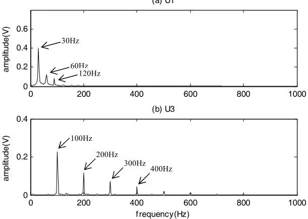
U1 and U3 are selected as fault components. The Hilbert envelope spectrum of U1 and U3 is shown in Figure 4.
0 200 400 600 800 1000
0 0.2 0.4 0.6
a
mp
lit
u
d
e
(V
)
(a) U1
0 200 400 600 800 1000
0 0.2 0.4
frequency(Hz)
a
mp
lit
u
d
e
(V
)
(b) U3
Figure 4.The Hilbert envelope spectrum of U1 and U3. 60Hz
As can be seen from Figure 4, in the envelope spectrum of the component U1, 2 times the
rotation frequency 60Hz and 4 times the rotation frequency 120Hz appear. There are many
interference frequencies in the envelope spectrum of the component U3, and the fault
features cannot be extracted effectively.In order to further extract the fault features, the fault
components are processed by RDT.The trigger value is set to 1.5 times the standard deviation
and the Hilbert envelope spectrum of the fault component is calculated, as shown in Figure 5.
0 200 400 600 800 1000 0
0.2 0.4 0.6
a
m
p
lit
u
d
e
(V
)
(a) U1
0 200 400 600 800 1000 0
0.2 0.4
f requency(Hz)
a
m
p
lit
u
d
e
(V
)
(b) U3
Figure 5.The Hilbert envelope spectrum of the fault components after RDT.
As can be seen from Figure 5, after the fault components are processed by RDT, the rotation frequency 30Hz, 2 times the rotation frequency 60Hz, and 3 times the rotation frequency 90Hz appear in the envelope spectrum of U1. The ignition frequency 100Hz, 2 times the ignition frequency 200Hz, 3 times the ignition frequency 300Hz and 4 times the ignition
frequency 400Hz appear in the envelope spectrum of U3.Therefore, the fault frequency and
its harmonics are successfully extracted, that is, the proposed method has successfully extracted the fault features from the simulation signal.
5.2 Experiment Condition
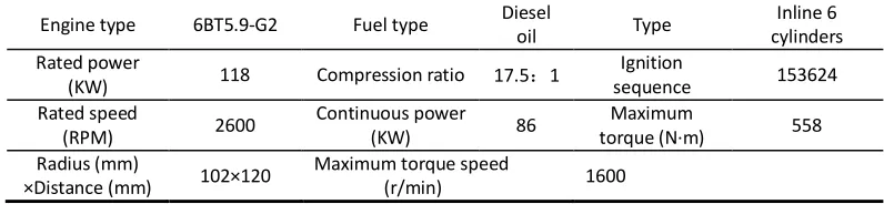
The structure of engine is complex and the working environment is abominable. As a result, it is prone to malfunction. The crankshaft bearing is located inside the engine, so it is difficult to diagnose the fault. In this paper, vibration signals are collected from the vibration sensors on the experimental stand, as shown in Figure 6. The basic parameters of the vibration sensor are shown in table 2. The engine on the experimental stand is Cummins 6BT diesel engine, and its parameters are shown in table 3.
60Hz 30Hz
120Hz
100Hz
200Hz 300Hz
Figure 6.Measuring position of vibration sensor.
Table 2. Vibration sensor parameters
Model Sensitivity Frequency range
(±3dB) Range Resolution
Temperature
range Weight
Output
connect
or 603C01 100mV/g 0.5Hz–10KHz ±50g 350μg -54-121℃ 51 g Top
Table 3. Basic parameters of the engine
Engine type 6BT5.9-G2 Fuel type Diesel
oil Type
Inline 6 cylinders Rated power
(KW) 118 Compression ratio 17.5:1
Ignition
sequence 153624 Rated speed
(RPM) 2600
Continuous power
(KW) 86
Maximum
torque (N·m) 558 Radius (mm)
×Distance (mm) 102×120
Maximum torque speed
(r/min) 1600
The fourth crankshaft bearings of Cummins EQ6BT engine are set with different clearance (0.10mm, 0.14mm, 0.20mm, 0.34mm) to simulate the normal, minor, moderate and severe wear of the connecting rod bearing. Vibration signals are collected on the left side of the fourth main bearings on the surface of the engine block. The sampling frequency is 20000Hz and the sampling points are 4096 points.
Testing temperature is important when acquiring vibration signals. In the experiment, the temperature of cooling water is measured to reflect the internal temperature of engine. The temperature is controlled at 60-70 degrees C.
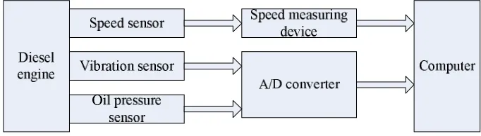
5.3 Data Acquired
The acquisition system is composed of collector, computer, sensor and connecting circuit,
as shown in Figure 7. According to document [28], the optimum diagnostic speed of this type
of engine is 1800r/min. In addition, four speeds were collected in the experiment: 800r/min, 1300r/min, 1800r/min, and 2100r/min. The experiment proved that 1800r/min is the most suitable for the fault diagnosis speed. Therefore, the acquisition system set the speed of the
engine to 1800r/min. Through the theoretical calculation, the rotation frequency of the crankshaft is about 30Hz, and the engine ignition frequency is about 90Hz.
Figure 7.Vibration signal acquisition system.
The vibration signals of the engine under different wear conditions are collected, as shown in Figure 8 and Figure 9. In Figure 8 and Figure 9, there is a large amount of background
noise in the vibration signals of different wear conditions of the the crankshaft bearing, which
is unfavorable to the extraction of fault features.
0 0.1 0.2 0.3 0.4 0.5 0.6 0.7 0.8 -5
0 5
(a) Normal w ear
a
m
p
lit
u
d
e
(V
)
0 0.1 0.2 0.3 0.4 0.5 0.6 0.7 0.8 -5
0 5
(b) Minor w ear
a
m
p
lit
u
d
e
(V
)
0 0.1 0.2 0.3 0.4 0.5 0.6 0.7 0.8 -5
0 5
(c) Moderate w ear
a
m
p
lit
u
d
e
(V
)
0 0.1 0.2 0.3 0.4 0.5 0.6 0.7 0.8 -5
0 5
(d) Severe w ear
time(s)
a
m
p
lit
u
d
e
(V
)
0 2000 4000 6000 8000 10000 0
500 1000
(a) Normal w ear
a
m
p
lit
u
d
e
(V
)
0 2000 4000 6000 8000 10000 0
500 1000
(b) Minor w ear
a
m
p
lit
u
d
e
(V
)
0 2000 4000 6000 8000 10000 0
500 1000
(c) Moderate w ear
a
m
p
lit
u
d
e
(V
)
0 2000 4000 6000 8000 10000 0
1000 2000
(d) Severe w ear
a
m
p
lit
u
d
e
(V
)
f requency(Hz)
Figure 9.The frequency domain waveform of vibration signal.
5.4 Experimental Data Processing
According to the proposed method, the VMD method is used to decompose the vibration signals under different wear conditions. The genetic algorithm is used to determine the
number of components [29]. According to the decomposition results of the vibration signals,
the permutation entropy of each component under different wear conditions is calculated respectively, as shown in table 4.
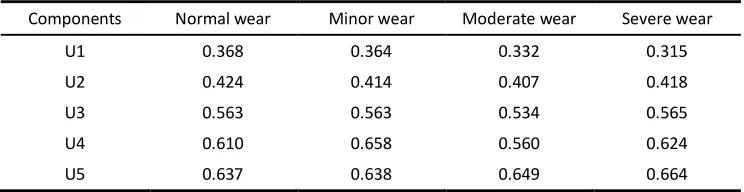
Table 4. The permutation entropy of each component under different wear conditions. Components Normal wear Minor wear Moderate wear Severe wear
U1 0.368 0.364 0.332 0.315
U2 0.424 0.414 0.407 0.418
U3 0.563 0.563 0.534 0.565
U4 0.610 0.658 0.560 0.624
U5 0.637 0.638 0.649 0.664
As we can see from Table 4, the permutation entropy values of the component U1 under different wear conditions are all the smallest, that is to say, the component U1 contains the most
abundant fault information.Therefore, the component U1 is selected as the fault component.
The Hilbert envelope spectrums of the component U1 under different wear conditions are
0 200 400 600 800 1000 0
0.5 1
(a) Normal w ear
a m p lit u d e (V )
0 200 400 600 800 1000 0
0.5 1
(b) Minor w ear
a m p lit u d e (V )
0 200 400 600 800 1000 0
0.5 1
(c) Moderate w ear
a m p lit u d e (V )
0 200 400 600 800 1000 0
0.5 1
(d) Severe w ear
a m p lit u d e (V ) frequency(Hz)
Figure 10.The Hilbert envelope spectrums of the component U1 under different wear conditions.
As can be seen from Figure 10, the characteristic frequency of the fault appears under the severe wear condition, and the characteristic frequency under the other wear conditions is not
obvious enough. With the increase of the clearance of the crankshaft, the energy of the
characteristic frequency point does not increase gradually.Therefore, the fault component is
further processed RDT, and its Hilbert envelope spectrum is shown as shown in Figure 11.
0 200 400 600 800 1000 0
0.1 0.2
(a) Normal w ear
a m p lit u d e (V )
0 200 400 600 800 1000 0
0.1 0.2
(b) Minor w ear
a m p lit u d e (V )
0 200 400 600 800 1000 0
0.1 0.2
(c) Moderate w ear
a m p lit u d e (V )
0 200 400 600 800 1000 0
0.1 0.2
(d) Severe w ear
a m p lit u d e (V ) frequency(Hz)
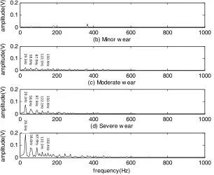
Figure 11.The Hilbert envelope spectrum of the fault components after RDT.
As can be seen from Figure 11, in the Hilbert envelope spectrum under different wear conditions, the rotation frequency, such as 29.3Hz, 58.6Hz, 122.1Hz, 151.4Hz, 210Hz and
ignition frequency, such as 87.9Hz and 180.7Hz, are found.With the increase of the clearance
of the crankshaft, the energy of the characteristic frequency point increases gradually.In order
to further illustrate the effect, the energy of the above characteristic frequency points in the Hilbert envelope spectrum is calculated respectively, as shown in Table 5.
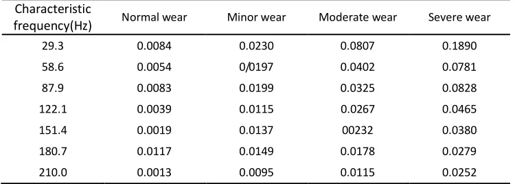
Table 5. The permutation entropy of each component under different wear conditions. Characteristic
frequency(Hz) Normal wear Minor wear Moderate wear Severe wear
29.3 0.0084 0.0230 0.0807 0.1890
58.6 0.0054 0/0197 0.0402 0.0781
87.9 0.0083 0.0199 0.0325 0.0828
122.1 0.0039 0.0115 0.0267 0.0465
151.4 0.0019 0.0137 00232 0.0380
180.7 0.0117 0.0149 0.0178 0.0279
210.0 0.0013 0.0095 0.0115 0.0252
As can be seen from Table 5, with the increase of the clearance of the crankshaft, the energy of the characteristic frequency point increases gradually, which is in accordance with the fault rule set by the test. The energy of the characteristic frequency point can reflect the vibration intensity of the engine. The greater the clearance of the crankshaft is, the stronger the impact of the engine. Therefore, according to the proposed method, the characteristic frequency of the engine crankshaft bearing fault is successfully extracted.
In order to further verify the advantages of VMD, the signal is processed in a similar way based on EMD and EEMD, as shown in Figure 12 and Figure 13.As can be seen from Figure 12 and Figure 13, fault feature cannot be effectively extracted based on EEMD and EMD, which shows the advantages of the proposed method.
0 200 400 600 800 1000
0 0.005 0.01
(a) Normal w ear
am
p
lit
u
de(
V
)
0 200 400 600 800 1000
0 0.005 0.01
(b) Minor w ear
a
m
pl
itude
(V
)
0 200 400 600 800 1000
0 0.005 0.01
(c) Moderate w ear
am
pl
itud
e(
V
)
0 200 400 600 800 1000
0 0.005 0.01
(d) Severe w ear
am
p
lit
u
de(
V
)
f requency(Hz)
0 200 400 600 800 1000 0
0.01 0.02
(a) Normal w ear
am
p
lit
u
de(
V
)
0 200 400 600 800 1000
0 0.01 0.02
(b) Minor w ear
a
m
pl
itude
(V
)
0 200 400 600 800 1000
0 0.01 0.02
(c) Moderate w ear
am
pl
itud
e(
V
)
0 200 400 600 800 1000
0 0.01 0.02
(d) Severe w ear
am
p
lit
u
de(
V
)
f requency(Hz)
Figure 13.Feature extraction method based on EEMD.
6 Conclusions
In the engineering application, the mechanical structure of the engine is very complex, which leads to the complex transmission path of the vibration signal. As a result, the excitation and response of multiple vibration sources are coupled to each other, which make the
diagnosis of crankshaft wear fault very difficult.In order to solve the above problems, a fault
feature extraction method for engine crankshaft bearing is proposed based on the variational
mode decomposition and random reduction technology.The research work of the simulation
signal analysis and the fault feature extraction of the crankshaft bearing are carried out. The conclusions are as follows:
(1) The proposed method can overcome the strong background noise, and successfully extract the rotation frequency and ignition frequency of the simulation signal.
(2) The proposed method is applied to the fault diagnosis of engine crankshaft bearing,
and the characteristic frequencies of crankshaft bearing fault under different wear conditions
are successfully extracted, which shows that the proposed method is effective. In addition,
compared with the method based on EMD and EEMD, the feature extraction result of the proposed method is better, which shows that the method is more advanced.
Acknowledgment
This work was funded by Key Project of the Army Equipment Department (Grant
no.WG2015JJ010008 ).
Conflicts of Interest
The authors declare that there are no conflicts of interest regarding the publication of
this paper.
References
1. Rauber T. W., Boldt F. D. A., et al. Heterogeneous Feature Models and Feature Selection Applied to
Bearing Fault Diagnosis. IEEE Transactions on Industrial Electronics. 2015, Vol.62, Issue 1, p.
637-646. [CrossRef]
2. Xie Z.J., Song B.Y., Zhang Y., Zhang F. Application of an Improved Wavelet Threshold Denoising
Method for Vibration Signal Processing. Advanced Materials Research. 2014, Issue 889-890, p.
799-806. [CrossRef]
3. HUANG N. E., SHEN Z., LONG S. R. The empirical mode decomposition and the Hilbert spectrum
fornonlinear and non-stationary time series analysis. Proceedings of the Royal Society. A. 1998,
Issue 454, p. 903-995.
4. HUANG N. E., SHEN Z., LONG S. R. A new view of non- linear water waves:The Hilbert spectrum.
Annu. Rev. Fluid Mech. 1999, Issue 31, p. 417-457.
5. Ai L., Wang J., Yao R. Classification of parkinsonian and essential tremor using empirical mode
decomposition and support vector machine. Digital Signal Process.2011, Vol. 21, Issue 4, p.
543-550. [CrossRef]
6. SU W.S., Wang F.T., Zhang Z.X., et al. Application of EMD denoising and spectral kurtosis in early
fault diagnosis of rolling element bearings. Journal of Vibration & Shock.2010, Vol. 22, Issue 1, p.
3537-3540.
7. Lahmiri., Boukadoum M. A weighted bio-signal denoising approach using empirical mode
decomposition. Biomed. Eng. Lett.2015, Vol. 5, Issue 2, p. 131–139.
8. Huang C,, Wang H., Long B. Signal Denoising Based on EMD. IEEE Circuits & Systems International
Conference on Testing & Diagnosis.2009, p. 1-4.
9. Zhang Y.K., Ma X.C., Hua D.X., et al. An EMD-based denoising method for lidar signal. International
Congress on Image & Signal Processing.2010, Issue 8, p. 4016-4019.
10. Khaldi K., Turki-Hadj Alouane M., et al. A new EMD denoising approach dedicated to voiced speech
signals. International Conference on Signals.2008, p. 1-5. [CrossRef]
11. Wang T., Zhang M., Yu Q., et al. Comparing the application of EMD and EEMD on time-frequency
analysis of seimic signal. Journal of Applied Geophysics, 2012, Vol. 83, Issue 6, p. 29-34.
12. WU Z. H., HUANG N. E. ENSEMBLE EMPIRICAL MODE DECOMPOSITION: A NOISE-ASSISTED DATA
ANALYSIS METHOD. Advances in Adaptive Data Analysis, 2005, Vol. 1, Issue 1, p. 0900004.
13. Wang H., Chen J., Dong G. Feature extraction of rolling bearing’s early weak fault based on EEMD
and tunable Q-factor wavelet transform. Mechanical Systems & Signal Processing, 2014, Vol. 48,
14. Dragomiretskiy K., Zosso D. Variational Mode Decomposition. IEEE Transactions on Signal
Processing.2013, Vol. 62, Issue 3, p. 531-544. [CrossRef]
15. Zhao C., Feng Z. P. Application of multi-domain sparse features for fault identification of planetary
gearbox. Measurement.2017, Issue 104, p. 169-179.
16. An X. L., Tang Y. J. Denoising of hydropower unit vibration signal based on variational mode
decomposition and approximate entropy. Transactions of the Institute of Measurement and
Control. 2016, Vol. 38, Issue 3, p. 282-292.
17. Li Z. P., Chen J. L., Zi Y. Y. Independence-oriented VMD to identify fault feature for wheel set
bearing fault diagnosis of high speed locomotive. Mechanical Systems and Signal Processing. 2017,
Issue 85, p. 512-529. [CrossRef]
18. E J. W., Bao Y. L., Ye J. M. Crude oil price analysis and forecasting based on variational mode
decomposition and independent component analysis. Physica A.2017, Issue 484, p. 412-427.
19. An X. L., Tang Y. J. Application of variational mode decomposition energy distribution to bearing
fault diagnosis in a wind turbine. Transactions of the Institute of Measurement and Control. 2017,
Vol. 39, Issue 7, p. 1000-1006.
20. Liu Y. Y., Yang G. L., Li M. Variational mode decomposition denoising combined the detrended
fluctuation analysis. Signal Processing.2016, Issue 125, p. 349-364. [CrossRef]
21. Yao J. C., Xiang Y., Qian S. C. Noise source identi- fication of engine based on variational mode
decomposition and robust independent component analysis. Applied Acoustics. 2017, Issue 116, p.
184-194. [CrossRef]
22. Cole H. A.On-the-line analysis of random vibration[C]//AIAA /ASME 9th Structure, Structural
Dynamics and Materials Conference, AIAA Paper, 1968: 268—288.
23. Cole H. A. Method and apparatus for measuring the damping characteristic of a structure: United
State, 3620069[P]. 1971.
24. Mikael A., Gueguen P., Bard P. Y., et al. The Analysis of Long-Term Frequency and Damping
Wandering in Buildings Using the Random Decrement Technique. Bulletin of the Seismological
Society of America, 2013, Vol. 103, Issue 1, p. 236-246. [CrossRef]
25. Yang J. C. S., Chen. J., Dagalakis N G. Damage detection in offshore structures by the Random
Decrement Technique. Journal of Energy Resources Technology, 1984, Vol. 55, Issue 106, p.
637-642. [CrossRef]
26. Bandt C., Pompe B. Permutation entropy: a natural complexity measure for time series.. Physical
Review Letters, 2002, Vol. 88, Issue 17, p. 174102.
27. Yan. R, Liu Y., Gao R. X. Permutation entropy: A nonlinear statistical measure for status
characterization of rotary machines. Mechanical Systems & Signal Processing, 2012, Vol. 29, Issue
5, p. 474-484. [CrossRef]
28. Xiao, Y., Mei, J., Zeng, R. Mechanical fault diagnose of diesel engine based on bispectrum and
Technology (pp.425-429). IEEE.
29. Li Y., Li H., Wang B., et al. Rolling Element Bearing Performance Degradation Assessment Using
Variational Mode Decomposition and Gath-Geva Clustering Time Series Segmentation.