An Efficient Path Detection And Direction Detection For Wsn
Shridhar.B.Chakalabbi student(M.tech), Department of ECE
Administrative Management College of Engineering 18th K.M, B G Road, Bengaluru, Karnataka, India Veena.S.K
Assistant Professor, Department of ECE
Administrative Management College of Engineering 18th K.M, B G Road, Bengaluru, Karnataka, India.
Abstract- The problem of tracking
signal-emitting mobile targets using navigated mobile
sensors based on signal reception. The Mobile Sensor
Collection node will initiate communication with
other sensor nodes in the network and finds multiple
measurements with respect to the target location and
then the time of arrival of each signal from the sensor
nodes is computed with respect to target by the
mobile sensor collector node . The path which has the
lowest TOA is said to be tagetory of the mobile node
in the network. But this project not only computes the
TOA but only measures the spatial separation with
respect to degrees so that the AOA of the mobile
target is also captured.
Keywords— Mobile sensor navigation, weighted tracking, TOA,crlb
1.INTRODUCTION
Wireless sensor networks (WSNs) are large
collections of small sensor devices that can be an
effective tool for collecting data from various
environments. Each sensor sends its data to Base
Station (BS), and finally BS sends these data to end
user. Clustering is considered as an effective
approach to provide better data gathering and
scalability for large sensor networks.
WIRELESS technologies have revolutionized the
world of communications. It started with the use of
radio receivers or transceivers for use in wireless
telegraphy early on; and now the term wireless is
used to describe technologies such as the cellular
networks and wireless broadband Internet. Although
the wireless medium has limited spectrum along with
a few other constraints as compared to the guided
media, it provides the only means of mobile
communication. Wireless ad hoc networking is used
for random and rapid deployment of a large number
of nodes, which is a technology with a wide range of
applications such as tactical communications, disaster
relief operations, health care and temporary
networking in areas that are not densely populated. A
mobile ad-hoc network (MANET) consists of mobile
hosts equipped with wireless communication devices.
The transmission of a mobile host is received by all
hosts within its transmission range due to the
broadcast nature of wireless communication and
omni-directional Sensore. If two wireless hosts are
not within the transmission range in ad hoc networks,
other mobile hosts located between them can forward
their messages, which effectively build connected
networks among the mobile hosts in the deployed
area. The use of wireless ad hoc networks also
introduces additional security challenges that have to
be dealt with.
2.Overview Of Mobile Sensor Navigation Strategy
In order to achieve the objectives of the project we
need the following modules
1. Node Deployment - This is responsible for placing the nodes in a given area
2. Coverage Area Determination - This module is used to determine the nodes which are
reachable or to which a given sensor node can communicate directly
3. Picking the Next Sensor - The next sensor is
picked randomly and target location is
determined with respect to given sensor
area.
4. Communicating the track or link - The tarck
of the target is send to mobile target
collector node through multiple paths.
5. Measuring the TOA - The TOA is measured
with respect to the distance of the node and
time of arrival of the detection packets.
6. Measuring the AOA - The angle of arrival of
the signals with respect to the target is
measured using kalman and CRLB approach
2.1 Maximum Margin Analyzer (MMA)
The Maximum Margin Analyzer is known as a
MMA. It is also alternatively a maximum likelihood
estimate of the power arriving from one direction
while all other sources are considered as interference.
Thus the goal is to maximize the Signal to
Interference Ratio (SIR) while passing the signal of
interest undistorted in phase and amplitude. The
source correlation matrix
R
ss is assumed to bediagonal. This maximized SIR is accomplished with
a set of array weights given by
)
(
)
(
)
(
1 1θ
θ
θ
a
R
a
a
R
w
xx H xx mma − −=
(2.30)Where,
R
xx−1 is the inverse of un-weighted arraycorrelation matrix
R
xxanda
(
θ
)
is the steering vectorfor an angle
θ
. The MMA pseudo spectrum is givenby
)
(
)
(
1
θ
θ
R
a
a
P
inv H
MMA
=
(2.31)
Where,
a
H(
θ
)
is the hermitian transpose ofa
(
θ
)
and
R
inv is the inverse of autocorrelation matrix.2.2 Kalman Method
This method finds a power spectrum such that its
Fourier transform equals the measured correlation
subjected to the constraint that its entropy is
maximized. For estimating TDD from the
measurements using an array of sensors, the Kalman
method finds a continuous function PRMEvR(θ) > 0 such
that it maximizes the entropy function.
The Kalman power spectrum is given by
)
(
)
(
1
θ
θ
E
E
a
a
P
Hs S H
KALMAN
=
Where,vectors
eigen
imum
E
s=
max
vector
steering
of
transpose
Hermitian
a
H(
θ
)
=
2.3 CRLB Filter
The goal of the CRLB []technique is to exploit the
rotational invariance in the signal subspace which is
created by two arrays with a translational invariance
structure. CRLB inherently assumes narrowband
signals so that one knows the translational phase
relationship between the multiple arrays to be used.
CRLB assumes that there are M< L narrow-band
sources centered at the center frequency f. M is
number of sources and L is the number of antenna
elements. These signal sources are assumed to be of a
sufficient range so that the incident propagating field
is approximately planar. The sources can be either
random or deterministic and the noise is assumed to
be random with zero-mean. CRLB assumes multiple
identical arrays called Doublets. Doublets can be
separate arrays or can be composed of sub arrays of
one larger array. It is important that these arrays are
displaced translation ally but not rotationally.
L element linear array is composed of two identical
(L-1) element sub-arrays or two doublets. These two
sub arrays are translational displaced by the distance
d as shown in Figure 2.6.
Fig: Doublet Representation
The target location can be computed as below
M
i
d
k
i
i
1
,
2
,
3
,....
)
(
tan
sin
1
1
=
=
− −λ
θ
Where,
d
is the distance between antenna elementsand
k
is the propagation constant2.4 Target Route Discovery Path1 Algorithm
The Individual Route Discovery Module is
implemented as shown in figure
Fig Individual Route Discovery Algorithm
The steps involved in the route discovery process is
as below
1. The wireless sensor node maintains a neighbor list,
which contains the ids of all nodes within its
transmission range.
2. It then randomly selects a neighbor for each share,
and uni-casts the share to that neighbor
3. The Process is repeated until the destination in
reached.
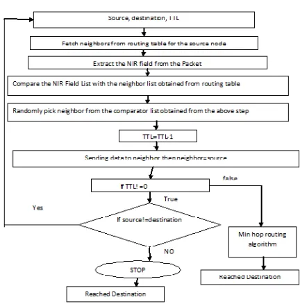
2.5 Route Discovery Path2 Algorithm
The Individual Route Discovery Module is
implemented as shown in figure
Fig: Individual Route Discovery Algorithm
The steps involved in the route discovery process is
as below
1. The wireless sensor node maintains a neighbor list,
which contains the ids of all nodes within its
transmission range.
2. When a source node wants to send shares to the
sink, it includes a TTL of initial value N in each
share
3. It then randomly selects a neighbor for each share,
and uni-casts the share to that neighbor
4. After receiving the share, the neighbor first
decrements the TTL.
5. If the new TTL is greater than 0, then compares the
neighbor list obtained from routing table with the list of nodes present in Node in Route (NIR Field).
6. After getting the set of nodes not present in NIR. The neighbor is randomly picked from the
neighboring nodes set not present in NIR and relays
the share to it, and so on .
6. When the TTL reaches 0, the final node receiving
this share stops the random propagation of this share,
and starts routing it toward the sink using normal
min-hop routing.
7. The Min-Hop Routing algorithm picks the farthest
node of its transmission range.
The minimum Hop Routing Algorithm used in the
algorithm when TTL becomes zero works as below
Min Hop routing algorithm picks the neighbor which
is closest to the destination node. ie farthest node
which is reachable.
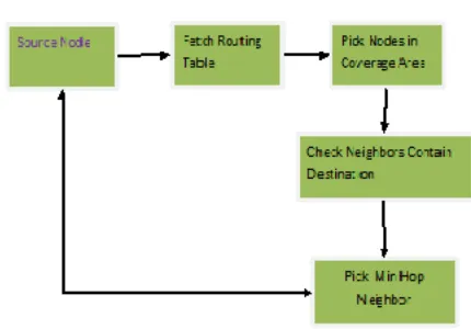
The Minimum Hop Routing algorithm is as shown in
figure
Fig Min Hop Routing Algorithm
Fig Shows the Minimum Hop Routing Algorithm. In
Minimum Hop Routing algorithm the source node
first fetches the routing table then fetches the
neighbors within transmission range. The Min Hop
Algorithm pick’s the intermediate node in such a way
that it is closest to the destination and farthest from
the source node.
3.Conclusion
[1] From the various simulations we can find out that
CRLB works best as compared to all other algorithms
for various cases like Low Sensors and Widely
spaced targets, Low Sensors and Closely Spaced
targets, Large Sensors and Widely Spaced targets and
finally Large sensor and Closely spaced sources.
[2] From the various simulations one can prove that
the TOA2 algorithm works better as compared to
TOA1 algorithm with respect to energy,time, power
and hops.
3.1 ACKNOWLEDGMENT
I am very much grateful to our college, the Dept. of
Digital Electronics And Communication Engineering
for providing me an opportunity for working on this
project. I express my sincere gratitude to my guide
Prof.VEENA.S.K for her guidance. Finally, I would
like to thank everyone who has directly or indirectly
helped me in this project.
4.References
[1] M. Cetin, L. Chen, J. Fisher, A. Ihler III, M.
Wainwright, and A.Willsky, “Distributed Fusion in
Sensor Networks,” IEEE SignalProcessing Magazine,
vol. 23, no. 4, pp. 42-55, Dec. 2006.
[2] A.H. Sayed, A. Tarighat, and N. Khajehnouri,
“Network-Based Wireless Location: Challenges
Faced in Developing Techniquesfor Accurate
Wireless Location Information,” IEEE Signal
Processing Magazine, vol. 22, no. 4, pp. 24-40, July
2005.
[3] N. Patwari, J.N. Ash, S. Kyperountas, A. Hero,
R.L. Moses, and N.S. Correal, “Locating the Nodes:
Cooperative Localization in Wireless Sensor
Networks,” IEEE Signal Processing Magazine,vol.
22, no. 4, pp. 54-69, July 2005.
[4] P.H. Tseng, K.T. Feng, Y.C. Lin, and C.L. Chen,
“Wireless Location Tracking Algorithms for
Environments with Insufficient Signal Sources,”
IEEE Trans. Mobile Computing, vol. 8, no. 12, pp.
1676-1689, Dec. 2009.[5] T. Li, A. Ekpenyong, and
Y.F. Huang, “Source Localization and Tracking
Using Distributed Asynchronous Sensors,” IEEE
Trans. Signal Processing, vol. 54, no. 10, pp.
3991-4003, Oct. 2006.
[6] L. Mihaylova, D. Angelova, D.R. Bull, and N.
Canagarajah,“Localization of Mobile Nodes in
Wireless Networks with Correlated in Time
Measurement Noise,” IEEE Trans. Mobile
Computing, vol. 10, no. 1, pp. 44-53, Jan. 2011.