R E V I E W
Open Access
Numerical simulations of multicomponent
ecological models with adaptive methods
Kolade M. Owolabi
*and Kailash C. Patidar
* Correspondence:
Department of Mathematics and Applied Mathematics, University of the Western Cape, Bellville 7535 Cape Town, South Africa
Abstract
Background:The study of dynamic relationship between a multi-species models has gained a huge amount of scientific interest over the years and will continue to maintain its dominance in both ecology and mathematical ecology in the years to come due to its practical relevance and universal existence. Some of its emergence phenomena include spatiotemporal patterns, oscillating solutions, multiple steady states and spatial pattern formation.
Methods: Many time-dependent partial differential equations are found combining low-order nonlinear with higher-order linear terms. In attempt to obtain a reliable results of such problems, it is desirable to use higher-order methods in both space and time. Most computations heretofore are restricted to second order in time due to some difficulties introduced by the combination of stiffness and nonlinearity. Hence, the dynamics of a reaction-diffusion models considered in this paper permit the use of two classic mathematical ideas. As a result, we introduce higher order finite difference approximation for the spatial discretization, and advance the resulting system of ODE with a family of exponential time differencing schemes. We present the stability properties of these methods along with the extensive numerical simulations for a number of multi-species models.
Results:When the diffusivity is small many of the models considered in this paper are found to exhibit a form of localized spatiotemporal patterns. Such patterns are correctly captured in the local analysis of the model equations. An extended 2D results that are in agreement with Turing typical patterns such as stripes and spots, as well as irregular snakelike structures are presented. We finally show that the designed schemes are dynamically consistent.
Conclusion:The dynamic complexities of some ecological models are studied by considering their linear stability analysis. Based on the choices of parameters in transforming the system into a dimensionless form, we were able to obtain a well-balanced system that is biologically meaningful. The accuracy and reliability of the schemes are justified via the computational results presented for each of the diffusive multi-species models.
Keywords:Coexistence, Competitive, Exponential time differencing, Predator-prey, Mutualism, Multistep methods, Reaction-diffusion systems, Stability analysis
AMS Subject Classification:Primary 70K05, 65M20, Secondary 70K20, 74H65
Background
The study of reaction-diffusion problems in ecological context have gained a huge amount of scientific interest, due to their practical relevance and emergence of some interesting phenomena such as spatial patterns, oscillating solutions, phase planes, cha-otic behaviours and multiple steady states to mention a few. The most popular and well-known predator-prey model is named after the two scientists, Alfred Lotka (1880– 1949) and Vito Volterra (1860–1940). Lotka and Volterra in their earlier research work apply the model to address the interacting population systems called predator–prey. Our numerical study in this paper is aimed at reflecting the types of interactions which we describe as predation (a process where one species of organisms called predator depends solely on the other known as the prey, for survival), competition (a situation whereby two or more different species of organisms struggle for the available resources; definitely, we expect the growth rate of each population to decrease) and lastly, the mutualism or symbiosis (organisms coexist without negatively affecting each other and hence, species growth rate is increased) [2, 11, 12, 23, 32, 33, 37, 39, 43, 48, 49].
A lot of research attention has been devoted to the study of population dynamics with regards to ecological interactions over the past few decades. Such studies include the predator-prey system that describes the situation in which the existence of the spe-cies called the predator depends solely on the other spespe-cies called the prey. The predator-prey system has received tremendous attraction over the years but has been represented mainly in terms of ordinary differential equations, which modelled the spe-cies distribution. The Dynamics of the Lotka-Volterra predator-prey model are quite interesting. However, this model is structurally unstable since a small perturbation of the equations often results to a drastic change in the dynamical system. For this reason, the presence of diffusion mechanism takes place though it changes the behavior of the whole model to coupled partial differential equations, called reaction-diffusion system. With the introduction of diffusion, the analysis of the whole system remain tactical in the literature [46, 47], and therefore, numerical approximations are quite often used to simulate these types of models.
Predator-prey systems have been studied by many researchers in various forms. For instance, in bacteria ecology, computer simulations of complex spatiotemporal patterns [4, 11] of Bacillus subtilis based on stochastic models [22] and deterministic models [29], Allee effect of patchy invasion on predator-prey dynamics [1, 3, 5, 7, 13, 39]. The diffusive predator-prey systems have also been studied extensively, see, [11, 17, 26, 27, 31, 38, 43]. Moreover, Wang et al. [46] investigated the spatial pattern formation of a predator-prey system with prey-dependent functional response of Ivlev type and reaction-diffusion whereas the analysis of predator-prey systems showing the Holling type II functional response is examined in Garvie and Trenchea [12].
model that each species has a different population of different sizes that grow logistic-ally in absence of each other and that each has a per capita growth rate that decreased linearly with the population size with their own intrinsic growth rate and carrying cap-acity. Mathematically, the simplest and instructive case is described by a system of two coupled-reaction diffusion equations. The system of two competing species in just one-dimensional space has attracted a lot of attentions, see [10, 14, 48] for details. Some of the evolution processes here are characterized owing to the fact that certain moments of time they experience a sudden change of state. To this end, we additionally consider a general case of $n$ competing species that is less investigated and still poorly under-stood for casen≥2. Among the few works done whenn> 2 include [37, 40, 43].
In mutualistic systems, organisms are found to evolve together. The existence of one has no negative effect on the other, each is part of the other's environment and co-exist, and they make use of each other in such a way that both organisms are benefited. Mutualism has not been given as much attention as predation and competition. Readers are referred to [20, 23] for a thorough review of the natural history of mutual-ism. Community invasion models have an issue of significant importance in the contemporary study of biological and ecological systems which have drawn the atten-tion of both theorists and ecologists since the foundaatten-tion work of Holt [18]. Despite a considerable achievements recorded in the field of population dynamics modeling the interaction of a multi-species community, so many challenging and open problems that are of great ecological importance are yet to be addressed.
Mathematical analysis of the main equations
In this work, our major attention is on the two-variable reaction-diffusion systems. We shall adapt linear stability analysis method to discuss the general two species dynamics. Letuandvbe the variables representing the two species of the Lotka-Volterra predator-prey type. In the convention here,vis the predator, whileurepresents the prey.
The most relevant and general two-species reaction-diffusion system is formulated as
∂u ∂t ¼Du
∂2u
∂x2þf uð ;vÞ; ∂v
∂t¼Dv ∂2v
∂x2þg uð ;vÞ;
)
ð1Þ
subject to zero-flux boundary conditions on a closed interval, say [0,L]
∂u ∂xð0;tÞ ¼
∂u
∂xðL;tÞ ¼0; ∂v
∂xð0;tÞ ¼ ∂v
∂xðL;tÞ ¼0:
)
ð2Þ
We assume that the point ð^u;^vÞ is stable equilibrium state of the homogeneous system
du
dt ¼f uð ;vÞ; du
dt ¼g uð ;vÞ; ð3Þ
J ¼ J11 J12 J21 J22
¼
∂F ∂u
ðu^;^vÞ
∂F ∂v
ðu^;v^Þ
∂G ∂u
ðu^;^vÞ ∂∂G
v
ðu^;^vÞ
0 B B B @
1 C C C
A ð4Þ
Which leads to characteristic equation of the formλ2−trJλ+ detJ= 0, where
trJ¼J11þJ22 <0; detJ ¼J11J22−J12J21>0: ð5Þ
To examine the stability of the uniform steady state ðu x^ð Þ;^v xð ÞÞ ¼ð Þ^u^v , we carry out the linear stability analysis in the spirit of Allen [2], Mendez et al. [28] and Murray [32, 33], we obtain
u xð ;tÞ^uþu0cosð Þkxeλkt; v xð ;tÞ^vþv0cosð Þkxeλkt;
)
ð6Þ
whereλk, the growth rates and the modes cos(kx) are the roots of polynomial
detðJ−D−InλkÞ ¼ J11−Duk 2−λ
k J12 J21 J22−Dvk2−λk
!
¼0;
ð7Þ
which corresponds to a polynomial
λ2
kþΦ1λkþΦ2 ð8Þ
representing the dispersion relation, with
Φ1¼ðDuþDvÞk2−trJ;
Φ2¼ J11−Duk2
J22−Dvk2
−J12J21¼DuDvk4−ðDvJ11þDuJ22Þk2þ detJ:
Known from the stability conditions in (5) thattrJ< 0, thus
Φ1¼ðDuþDvÞk2−trJ <0;∀k:
Which shows that the uniform steady state of (1) cannot undergo an oscillatory in-stability (or wave bifurcation) to a standing wave pattern.
A Turing instability corresponds to λktrJ ¼0 for ktrJ≠0. That is, with Φ2= 0, results
to (J11−Duk2)(J22−Dvk2)−J12J21= 0 or
k4− J11 Du
þJ22 Dv
k2þ detJ DuDv
¼0 ð9Þ
For the roots of (9) to be positive,
DvJ11þDuJ22 >0 ð10Þ
is a necessary but not sufficient condition for the Turing instability to occur. With ref-erence to conditions in (5), Turing instability can occur if the diffusion coefficientDu≠
Dv and if the matrix elements J11 and J22 have opposite sign. So, Turing instabilities occur only in either pure or cross activator-inhibitor dynamical system.
J ¼ þþ −−
; for J11 >0;J22 <0;J12<0;J21>0 ð11Þ
Again, it is of thecrossLotka-Volterra type if the Jacobian has the structure
J ¼ þ þ− −
; for J11>0;J22<0;J12>0;J21<0 ð12Þ
Clearly from systems (11) or (12), we haveJ11> 0,J22< 0 which together with DvJ11+ DuJ22> 0 indicates that Turing instability can occur only if |J22| >J11 since trJ< 0 and J12J21< 0 for detJ> 0. If we let ΘD=Dv/Du be the diffusion coefficients ratio, we can
easily obtain from (10) that ΘD>J22/J11> 1. The indication here is that, for Turing in-stability to take place, the inhibitor must diffuse faster than the activator.
By rewriting (9) in the form
k4þΨ1k2þΨ2¼0;
where
Ψ1 ¼− J11 Du
þJ22 Dv
; Ψ2¼ detJ DuDv;
we have the roots of equation (9) given by
k21;2¼−Ψ1
2
ffiffiffiffiffiffiffiffiffiffiffiffiffiffiffiffiffiffi
Ψ2 1−4Ψ2
q
2 ;
providedΨ1< 0 and condition (10) is satisfied. So, Turing instability occurs for (10) to have a double root, that is, ifΨ12−4Ψ2= 0.
In conclusion, the uniform steady state of the reaction-diffusion system (1),
^
u xð Þ;^v xð Þ
ð Þ ¼ð Þu^^v , that satisfy the stability conditions in (5) will be unstable in the presence of diffusion (called diffusion driven-instability) ifΨ1< 0, that is,DvJ11+DuJ22> 0, and Ψ12−4Ψ2> 0, that is, (DvJ11+DuJ22)2> 4DuDvdetJ, with the band of unstable
modes
−Ψ1−
ffiffiffiffiffiffiffiffiffiffiffiffiffiffiffiffiffiffi
Ψ2 1−4Ψ2
q
2
0 @
1
A<k2< −Ψ1þ
ffiffiffiffiffiffiffiffiffiffiffiffiffiffiffiffiffiffi
Ψ2 1−4Ψ2
q
2
0 @
1
A:
A good research focus has to be given to the numerical simulation of multi-species dynamics in more than one dimensional space which has received little attention in the literature. We simulated a class of biological systems that lead to the evolution of traveling waves and formation of chaotic and spatiotemporal patterns arising in the context of mathematical ecology. Though, simulations that are based on the use of conventional methods in two-dimensions are found to be time consuming. As a result, consideration is given to the design and method of implementing a viable numerical scheme that can handle a class of multi-component reaction-diffusion problems efficiently.
Numerical methods
∂w ∂t ¼D∇
2wþN wð ;tÞ ð13Þ
where D> 0 is the diffusion coefficient, ∇2w= (∂2w/∂x2+∂2w/∂y2) is the two-dimensional Laplacian operator that represents the linear term, and N is nonlinear function of w and t. By following [34–36], we discretize the spatial domain by mesh (xi,yj) = (T1+i×hx,T1+j×hy) where hx= (T2−T1)/(Nx+ 1), hy= (T2−T1)/(Ny+ 1), for 0≤i≤Nx+ 1, 0≤j≤Ny+ 1. We approximate the second-order derivatives by the fourth-order central difference operators
∂2w ∂x2 ¼
−wi−2;jþ16wi−1;j−30wi;jþ16wiþ1;j−wiþ2;j
12h2x ¼L1;
∂2w ∂y2 ¼
−wi;j−2þ16wi;j−1−30wi;jþ16wi;jþ1−wi;jþ2
12h2y ¼L2;
and
w¼
wi;j wi;jþ1 ⋯ wi;Nyþ1
wiþ1;j wiþ1;jþ1 ⋯ wiþ1;Nyþ1
⋮ ⋮ ⋮ ⋮
wNx;j wNx;jþ1 ⋯ wNx;Nyþ1
0 B B @
1 C C A
NnNyþ1
for i= 1, 2,…,Nx and j= 1, 2,…,Ny+ 1. The discretized form of (13) lead to a coupled system ordinary differential equations (ODEs)
dw
dt ¼D Lð 1þL2ÞwþN wð ;tÞ ð14Þ
whereL1,L2∈Landw=w(u,v).
Exponential integrators separate the linear term involving L, which is solved exactly by a matrix exponential, from the nonlinear term. The theory of numerical methods for the time integration of semi-linear problems has been proposed by the application of the exponential methods. Cox and Matthews [6] presented derivation of exponential time differencing (ETD) methods. Few years later, a modification of the ETD Runge-Kutta methods of Cox and Matthews was made by Kassam and Trefethen [21], and it is from their paper that we present some details of the scheme. A new algorithm for the implementation of the exponential methods has been discussed in [9], that the al-gorithm evaluates the operator by the exponential methods with a quadrature formula that converges. Hochbruck and Ostermann [15] discussed further on the class of expli-cit multistep exponential and expliexpli-cit exponential Runge-Kutta methods. In this paper, we use both the fourth-order exponential time differencing Runge-Kutta method [6, 21] and the fourth-order exponential multistep method of Adams-type [6, 16].
Exponential time differencing method
w tnð þ1Þ ¼w tnð ÞeLΔtþeLΔt
ZΔt
0
e−LτN w tnð ð þτÞ;tnþτÞdτ ð15Þ
This equation is known to be exact [6, 21]. Various ETD schemes come from how one approximates the integral on the right hand side in the above equation. The article by Cox and Matthews [6] contains various approximations to the integral. They first presented the sequence of recurrence formulae that give higher-order approximations of a multistep method of Adams-type. In their work, a general ETD scheme of order-s was proposed as
wnþ1¼wneLΔtþΔt
Xs−1
j¼0 gjX
j
k¼0 −1
ð Þk j
k Nn−k: ð16Þ
The coefficients gjare obtained by the recurrence relation
LΔtg0¼eLΔt−1;
LΔtgjþ1þ1¼gjþ1
2gj−1þ 1
3gj−2þ⋯þ 1
jþ1g0¼
Xj
k¼0 1
jþ1−kgk:
ð17Þ
By setting s= 4 in the explicit integrating formula (16), we obtain the fourth-order ETD scheme of Adams-type
wnþ1¼wneLΔtþðΘ1Nn−Θ2Nn−1þΘ3Nn−2−Θ4Nn−3Þ= 6L2Δt3
; ð18Þ
where
Θ1¼ 6L3Δt3þ11L2Δt2þ12LΔtþ6
eLΔt−24L3Δt3−26L2Δt2−18LΔt−6;
Θ2¼ 18L2Δt2þ30LΔtþ18
eLΔt−36L3Δt3−57L2Δt2−48LΔt−18;
Θ3¼ 6L2Δt2þ24LΔtþ18
eLΔt−24L3Δt3−42L2Δt2−42LΔt−18;
Θ4¼ 2L2Δt2þ6LΔtþ6
eLΔt−6L3Δt3−11L2Δt2−12LΔt−6;
denoted in this paper as ETDADAMS4.
Similarly, Cox and Matthews derived a set of ETD schemes that are based on Runge-Kutta time-stepping, which they call ETDRK schemes. We only use the fourth-order scheme which we denoted as ETDRK4 in this paper. On setting s= 4 again in (16), we have the ETDRK4 formula
wnþ1¼wneLΔtþNn −4−LΔtþeLΔt 4−3LΔtþL2Δt2
þ2ðN að n;tnþΔt=2Þ þN bð n;tnþΔt=2ÞÞ 2þLΔtþeLΔtð−2þLΔtÞ
þN cð n;tnþΔtÞ −4−3LΔt−L2Δt2þeLΔtð4−LΔtÞ
=L3Δt2;
ð19Þ
where
an¼wneLΔt=2þeLΔt=2−INn=L; bn¼wneLΔt=2þ eLΔt=2−I
N að n;tnþΔt=2Þ=L; cn¼wneLΔt=2þeLΔt=2−Ið2N bnð ;tnþΔt=2Þ−NnÞ=L:
φð Þ ¼L 1
2πi
Z
Γφð Þt ðtI−LÞ
−1
dt; ð20Þ
to evaluate the coefficients of these schemes. Further details on derivations and applica-tions of ETD Adams-type and ETD Runge-Kutta methods can be found in [6,21,41].
Stability analysis
We investigate the stability of the fourth-order ETDADAMS4 (18) and ETDRK4 (19) schemes by linearizing the nonlinear autonomous system [8, 19]
dw tð Þ
dt ¼Lw tð Þ þN w tð ð ÞÞ; ð21Þ
withN(w(t))the nonlinear part. We suppose that there exists a fixed pointw0such that
Lw0+ N(w0)= 0. Linearizing about this fixed point, we obtain
dw tð Þ
dt ¼Lw tð Þ þλw tð Þ; ð22Þ
where w(t)is now the perturbation ofu0and λ=N′(w0) is a diagonal or a block diag-onal matrix containing the eigenvalue of N. In an attempt to keep the fixed point u0 stable, we require that Re(L+λ) < 0, for allλ. It is naturally important for a numerical method to satisfy this property so as to cover as much dynamics as possible.
When applying ETDADAMS4 (18) to the linearized problem (22), a polynomial equation of the order-four inris obtained in the form
w4r4þw3r3þw2r2þw1rþw0¼0; ð23Þ
where
w0¼ ½ð2y2þ6yþ6Þey−6y3−11y2−12y−6x;
w1¼ ½ð−9y2−24y−18Þeyþ24y3þ42y2þ42yþ18x; w2¼ ½ð18y2þ30yþ12Þey−36y3−57y2−48y−18x;
w3¼−6y6eyþ ½ð−6y3−11y2−12y−6Þeyþ24y3þ26y2−18yþ6x; w4¼6y4:
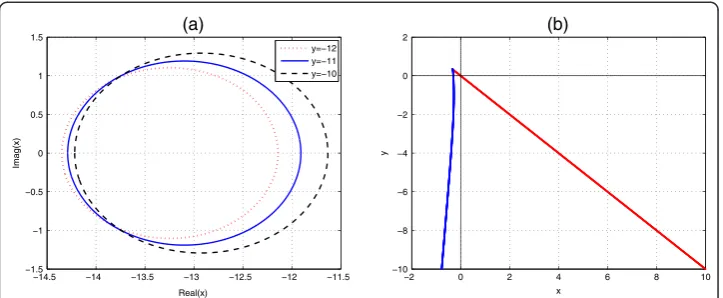
In the real (x, y) plane, the right-hand boundary for ETDADAMS4 scheme corre-sponds to substituting r= 1 in equations (23) is the line x + y= 0. The corresponding left-hand boundary for substitutingr=−1, also in (23), is given by the curve
x¼ 3y
4ðeyþ1Þ
3y3þ20y2þ36yþ24
ð Þey−45y3−68y2−60y−24 ð24Þ
as displayed in Fig.1.
In a similar fashion, the application of ETDRK4 method (19) to the linearized prob-lem (22) leads to a recurrence relation
r¼wnþ1
wn ¼L0þL1xþL2x 2þL
3x3þL4x4; ð25Þ
L0¼ey
L1¼− 4
y3þ 8ey=2
y3 − 8e3y=2
y3 þ 4e2y
y3 − 1
y2þ 4ey=2
y2 − 6ey
y2 þ 4e3y=2
y2 − e2y
y2
L2¼− 8
y4þ 16ey=2
y4 − 16e3y=2
y4 þ 8e2y
y4 − 5
y3þ 12ey=2
y3 − 10ey
y3 þ 4e3y=2
y3
−e2y y3 −
1
y2þ 4ey=2
y2 − ey=2
y2
L3¼ 4
y5− 16ey=2
y5 þ 16ey
y5 þ 8e3y=2
y5 − 20e2y
y5 þ 8e5y=2
y5 þ 2
y4− 10ey=2
þ16ey
y4 − 12e3y=2
y4 þ 6e2y
y4 − 2e5y=2
y4 − 2ey=2
y3 þ 4ey
y3 − 2e3y=2
y3
L4¼ 8
y6− 24ey=2
y6 þ 16ey
y6 þ 16e3y=2
y6 − 24e2y
y6 þ 8e5y=2
y6 þ 6
y5− 18ey=2
y5
þ20ey
y5 − 12e3y=2
y5 þ 6e2y
y5 − 2e5y=2
y5 þ 4
y4− 6ey=2
y4 þ 6ey
y4 − 2e3y=2
y4 ;
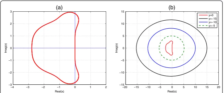
where x=λh, y=Lh. We can define the amplification factor for ETDRK4, r(x, y)
for y >0. If y = 0, the amplification factor becomes 1−x+x2/2−x3/6 +x4/24. Hence, we can see that the stability curve of ETDRK4 at y= 0 coincides with that of the classical fourth-order Runge-Kutta method, Fig. 2(a). We also see that limx,y→0∂xr(x,y) =−1 and limx,y→0∂yr(x,y) =−1. Hence, the absolute value of the amplification factor is given as |r(x,y)|≤1.
The boundary of the stability region can be determined by settingr=eiθ, forθ∈[0, 2π]. We plot the stability region in the complex x plane and displayed in Fig. 2, where the horizontal and vertical axes represent the real and imaginary ofx, respectively.
Numerical examples and results
In this section, numerical methods we discussed above are now applied to the three major classes of the Lotka-Volterra two-species models. In addition, comparison with other adaptive methods are made to justify the effectiveness and accuracy of the present method. A possible extension to two space dimensions is considered, since it is in higher dimensions that most of the ideas reported are of serious value.
−14.5 −14 −13.5 −13 −12.5 −12 −11.5 −1.5 −1 −0.5 0 0.5 1 1.5 Real(x) Imag(x) (a) y=−12 y=−11 y=−10
−2 0 2 4 6 8 10
−10 −8 −6 −4 −2 0 2 x y (b)
Predator-prey system
It is clear from our introduction that predator-prey models are similar in description to both parasite and parasitoid models. A typical example of predator-prey model [11, 32] is the reaction-diffusion system
∂U ∂T ¼D1∂
2U
∂X2þU α 1− U K
0 @
1
A− γV
Uþδ
2 4
3
5;
∂V ∂T ¼D2
∂2V
∂X2þV β 1− hV
U
0 @
1 A 2
4
3
5;
)
ð26Þ
whereUandVare the densities of the prey and predator respectively,D1> 0 andD2> 0 are diffusion coefficients for the prey and predator.α,β,γ,δ,handKare positive parameters. The term αU(1−U/K) represents the logistic growth,α is the intrinsic growth rate, and Kthe carrying capacity. The termγVis the per-capita prey reduction due to consumption by the predator, andβdescribes the intensity of predation.
To reduce the number of parameters in (26), we nondimensionalize the model by re-scaling the variables as
u tð Þ ¼U Tð Þ
K ; v tð Þ ¼ hV Tð Þ
K ; t¼αT; μ¼ γ hα; ψ¼
β α; φ¼
δ K; D¼
D2 D1
ð27Þ
to yield
∂u ∂t ¼
∂2u
∂x2þuð1−uÞ−
μu
uþφv¼f uð ;vÞ; ∂v
∂t¼D ∂2v ∂x2þψv−
ψv2
u ¼g uð ;vÞ:
)
ð28Þ
For the linear stability, we have to analyze the stability criteria of the non-diffusive system [17, 31, 42]. The spatial model (28) has the corresponding non-diffusive systems
−4 −3 −2 −1 0 1 2
−3 −2 −1 0 1 2 3
Real(x)
Imag(x)
(a)
−20 −15 −10 −5 0 5 10 15 20
−15 −10 −5 0 5 10 15
Real(x)
Imag(x)
(b)
y=0 y=−15 y=−10 y=−5
du
∂t ¼uð1−uÞ− μu
uþφv¼f uð ;vÞ; dv
∂t ¼ψv− ψv2
u ¼g uð ;vÞ;
)
ð29Þ
with just three parametersμ> 0,ψ> 0 andφ> 0. There are other choices for the change of var-iables to put the system in dimensionless form, but we opt for the choice that suits our purpose since the dimensionless groupings used here give relative measures of the effect of dimensional parameters. For instance, ' now becomes the ratio of the linear growth rate of the predator to that of the prey, forψ< 1. We expect the prey to reproduce faster than the predator otherwise the system will go into extinction.
At equilibrium, fð Þ ¼^u^v gð Þ ¼u^^v 0 , since the steady state populations û and ^v are solutions ofdu/dt = dv/dt= 0. Hence,
^
uð1−^uÞ− μu^
uþφ^v¼0; ψ^v−ψ^v2u^¼0:
)
ð30Þ
Naturally, for the dynamical system under consideration to be biologically meaningful, we should have both u≥0,v≥0 at all times. We observe from (30) that the system (28) has three positive steady states ð Þu^^v , the two trivial states or saddle points are at point (0, 0) which describes complete extinction of both prey and predator and point (1, 0), which shows that the predator is absent leading to unbounded logistic growth of the prey species. The stationary point ð Þu^^v corresponding to the existence of predator and prey, bearing in mind that for the system under consideration to be biologically meaningful, the parameters must be strictly restricted to the positive quadrants, gives
^
u¼^v¼ð1−μ−φÞ þ ð1−μ−φÞ 2þ
4φ
1=2
2 : ð31Þ
The stability of the steady or equilibrium states are the singular points in the phase plane of (28). To determine them, we let
A¼ ^u μu^ ^ uþφ
ð Þ2−1
2 4
3
5 −μu^
^ uþφ
ψ −ψ
0 B @
1 C
A; ð32Þ
whereAis regarded as the community matrix with eigenvalues given by
A−λI
j j ¼0⇒λ2−ðtrAÞλþ detA¼0: ð33Þ
For stability, we require that Reλ< 0. Hence, the necessary and sufficient conditions for linear stability become
trA<0 ⇒ ^u μu^−ðu^þφÞ 2
^ uþφ
ð Þ2
2 4
3
5<ψ
detA>0 ⇒ ðu^þφÞ 2þμ ^
uþφ
ð Þ−μu^ ^
uþφ
ð Þ2 >0:
)
ð34Þ
Results in one-dimension for system (26)
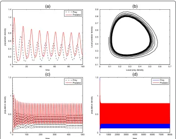
Numerical results of the predator-prey system are shown in one-dimension. The initial data and parameter values are given in the figure caption. The initial data are chosen as a result of small perturbations of the steady state solutions û and ^v of the spatially homogeneous system. By varying the choice of parameters lead to different spatial pat-terns, such as oscillatory smooth, intermittent structure and spatiotemporal patterns. It should be noted that other one-dimensional spatial structures that are not captured here are possible, depending on the choice of the parameter values and initial data.
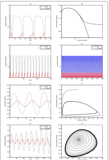
Figures 3 and 4 represent the unrealistic and realistic population dynamics of the predator-prey systems. The system with nonlinear part as described in Garvie [11] is quite unrealistic due to the choices of parameters used in transforming the system into a dimensionless form. This shortcoming actually motivates us to choose some appropriate parameters since it is always helpful to write the system in nondimensional form. Non-dimensionalisation plays an important role when carefully considered because it reduces the number of parameters by grouping them in a more meaningful manner. So, the system described in Fig. 3 is totally unrealistic as it is prone to danger of extinction of the prey species that would in turn results to total breakdown of the ecosystem since all the predators will die out in absence of food. In Fig. 4, spatiotemporal oscillations arise and population oscillations are transient and regular. It should be noted that due to the formation of spatial pattern, the two species can dynamically coexist.
0 20 40 60 80 100
0 0.2 0.4 0.6 0.8 1 1.2 1.4
time
population density
(a)
Prey Predator
0 0.1 0.2 0.3 0.4 0.5 0.6 0.7 0.1
0.2 0.3 0.4 0.5 0.6 0.7 0.8 0.9
Local prey density
Local predator density
(b)
0 100 200 300 400 500
0 0.5 1 1.5
time
population density
(c)
Prey Predator
0 1000 2000 3000 4000 5000 6000 7000 8000 0
0.5 1 1.5
time
population density
(d)
Prey Predator
Results in two-dimension for system (26)
We intend to mimic the two-dimensional results obtained for the predator-prey system in [11, 27], we experiment with the same initial data
0 50 100 150 200 250 300 350 400 0
0.5 1 1.5
time
population density
(a)
Prey Predator
0 0.5 1 1.5
0 0.05 0.1 0.15 0.2 0.25
Local prey density
Local predator density
(b)
0 500 1000 1500
0 0.5 1 1.5
time
population density
(c)
Prey Predator
0 1000 2000 3000 4000 5000 6000 7000 8000 0
0.5 1 1.5
time
population density
(d)
Prey Predator
0 20 40 60 80 100
0.32 0.33 0.34 0.35 0.36 0.37 0.38 0.39 0.4 0.41
time
population density
(e)
Prey Predator
0 0.1 0.2 0.3 0.4 0.5 0.6 0.7 0.8 0.9 0.05
0.1 0.15 0.2 0.25 0.3 0.35 0.4
Local prey density
Local predator density
(f)
0 50 100 150 200 250 300
0.3 0.32 0.34 0.36 0.38 0.4 0.42
time
population density
(g)
Prey Predator
0.2 0.25 0.3 0.35 0.4 0.45 0.5 0.55 0.3
0.31 0.32 0.33 0.34 0.35 0.36 0.37 0.38 0.39
Local prey density
Local predator density
(h)
u xð ;y;0Þ ¼u^−ð210−7Þðx−0:1y−225Þðx−0:1y−675Þ; v xð ;y;0Þ ¼^v−310−5ðx−450Þ−ð1:210−4Þðy−150Þ
ð35Þ
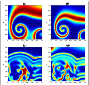
so as to induce a nontrivial spatiotemporal dynamics of the homogeneous stationary states û and ^v. In Fig. 5, numerical simulations was done on a square domain size [0, 700] × [0, 700], with parameter values D= 0.1, μ= 0.2, ψ= 2, φ= 0.5 at non-trivial state ð Þu^^v =(6/35, 116/245). As simulation time is increased from t= 200 to
t= 500, the spiral patterns in (a, b) are disjointed and spreads out in the domain to form a stripe-like structures with emergence of some spots underneath. It should be mentioned that if the simulation time is further increased, say to
t= 1500 and above, there is every tendency of getting a Turing and more compli-cated spatiotemporal patterns. In addition, we realized that the choice of initial conditions can influence the type of spatiotemporal dynamics of a reaction-diffusion problem in ecosystems.
A close look at the first and second columns in Fig. 5 have revealed that both predator and prey species have a similar distribution. As a result, our pattern forma-tion analysis is henceforth restricted to only one distribuforma-tion. We also observe in our experiments that increase in domain size actually results to increase in
computational time. Henceforth, we choose to simulate with a smaller square domain of size [0, 250] × [0, 250].
Competitive system
Competition model describes a situation in which two or more species compete for the same (sufficient or insufficient) resources like food, territory or in some way inhibit each other of growth. For simplicity, and by following the approach we used for the predator-prey model, we consider here the two-species Lotka-Volterra competition model
∂U ∂T ¼δ1∂
2U
∂X2þα1U 1− U K1−β1
V K1
0 @
1
A;
∂V ∂T ¼δ2
∂2V
∂X2þα2V 1− V K2−β2
U K2
0 @
1
A;
)
ð36Þ
with species Uand Vhaving logistic growth in the absence of the other. The parame-ters α1 and α2 represent their linear birth rates, β1 and β2 measure the competitive effect ofVonUand vice versa,δ1and δ2stand for the diffusion coefficients of species
UandV, andK1andK2are their respective carrying capacities.
Again, we nondimensionalize (36) by introducing a set of carefully selected dimen-sionless variables
u tð Þ ¼U Tð Þ K1 ;
v tð Þ ¼V Tð Þ K2 ;
t¼α1T; μ¼αα2 1; φ
¼β2 K2 K1; ψ
¼β1 K1 K2; δ
¼δ2
δ1:
ð37Þ
As suggested by Medvinsky et al. [27] and Garvie [11], the local stability analysis will always grant a deeper understanding and will provide important information on the choice of parameters for numerical integration. Like the previous case, we continue with the local stability analysis in the absence of diffusion. Using (37) in (36), we obtain
∂u ∂t ¼
∂2u ∂x2þ u−u
2−φuv
¼f uð ;vÞ;
∂v ∂t¼δ
∂2v
∂x2þμ v−v 2−ψuv
¼g uð ;vÞ:
)
ð38Þ
For the linear stability analysis, we consider the case of spatially homogeneous solu-tions, in which the spatial model (38) is equivalent to the system of ordinary differential equations
du
∂t ¼ u−u 2−φuv
¼f uð ;vÞ;
dv
∂t ¼μ v−v2−ψuv
¼g uð ;vÞ:
)
ð39Þ
Here, we regard the steady states and phase plane singularities,û and ^v as the solu-tions off(u,v)= g(u, v) = 0. This gives four positive equilibrium states,
^ u;^v
ð Þ ¼ð0;0Þ; ð^u;^vÞ ¼ð1;0Þ; ðu^;^vÞ ¼ð0;1Þ; ðu^;^vÞ ¼ 1−φ
1−φψ; 1−ψ 1−φψ
: ð40Þ
The first three stationary states are trivial whereas the last one is non-trivial. The state (0,0) corresponds to total washout state of the two species, the second state (1,0) stands for the ex-istence and extinction of species u and v respectively and the third trivial state (0; 1) indicate that only species v will exist. It is obvious that none of the three trivial states could give a meaningful interpretation about the competition model, therefore, there is the need to explore further the nontrivial equilibrium stateðu^;^vÞ. The points (0,0), (1,0) and (0,1) are all unstable (0,0) is an unstable node, (1,0) and (0,1) are saddle point equilibria. From (39), for f = g =0, we have that (u−u2−φuv) = 0, it follows that eitheru =0 or 1−u− −φv= 0 and also from the second equation,μ(v−v2−φuv) = 0 which implies,μv= 0 and 1−v− −φu= 0.
Now the Jacobian or community matrix for this system evaluated atðu^;^vÞis
A¼ 1−−2μψu−φv −φu v μð1−2v−ψuÞ
^
u;^v
ð Þ:
ð41Þ
The point (0, 0), is unstable since the eigenvaluesλobtained from
A−λI
j j ¼ 1−λ 0
0 μ−λ
¼0
areλ1,2= (1,μ). At the point (1, 0), the community matrixAgives
A−λI
j j ¼ 1−λ φ
0 μð1−ψÞ−λ
¼0:
Hence, λ1,2= (−1,μ(1−ψ)). Therefore, the steady state ðu^;v^Þ ¼ð1;0Þis stable ifψ> 1 and unstable otherwise. In the same manner, we can see that the steady state (0, 1) has the community matrixAsatisfying
A−λI
j j ¼ð1−μφφÞ−λ −μ0−λ¼0:
The corresponding eigenvalues are λ1,2= (−μ, (1−φ)). This means that the steady stateðu^;^vÞ=(0, 1) is stable ifφ> 1 and unstable ifφ< 1.
For the fourth steady states, we have matrix,
A−λI
j j ¼
1−2 1−φ 1−φψ
0 @
1
A−φ 1−ψ
1−φψ
0 @
1 A 2
4
3
5−λ −φ 1−φ
1−φψ
−μ 1−ψ
1−φψ −μ 1−2
1−ψ 1−φψ
0 @
1
A−ψ 1−φ
1−φψ
0 @
1 A 2
4
3
5−λ
¼0:
The eigenvalues in this case are
λ1;2¼
φ−1
ð Þ þμ ψð −1Þ
ffiffiffiffiffiffiffiffiffiffiffiffiffiffiffiffiffiffiffiffiffiffiffiffiffiffiffiffiffiffiffiffiffiffiffiffiffiffiffiffiffiffiffiffiffiffiffiffiffiffiffiffiffiffiffiffiffiffiffiffiffiffiffiffiffiffiffiffiffiffiffiffiffiffiffi
φ−1
ð Þ þμ φð −1Þ2
−4μð1−φψÞðφ−1Þ2
q
2 1ð −φψÞ :
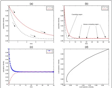
intersection of the isoclines regardless of the initial population densities. The intersec-tion point of the two lines gives the positive steady state as in (a) where the point (1.4, 1.4) corresponds to (1/φ, 1/ψ). The locations of the isoclines in (b) dictate that species u out-competes species v, the point (1/φ, 1/ψ) corresponds to the value (1.6, 0.6) of species u and v, respectively. Clearly, on rearranging, we can see that ψ<K2/K1 and φ<K1/K2, and these competition coefficients must be made as small as possible relative to the ratio of its carrying capacity to that of other species. These conditions must hold for both species simultaneously, and this is possible only if the carrying capacities of the two species are similar in such a way that their ratio is close to one. Figure 7 (a) describes the species declining population density asso-ciated with the competitive system (38), panels (b,c) refer to the time series solu-tion, and (d) corresponding to the species phase plane diagram.
Two dimensional results for model (38)
We also carry out a two-dimensional numerical simulations of the spatially extended competitive model (38). We employed the initial conditions (35) and the zero-flux boundary conditions on a square domain size of [0, 250] × [0, 250] with time-step Δt = 0.005 and grid widthΔh =0.25. Here the parameter values are set as
δ¼0:05; φ¼0:2; ψ¼0:69; μ¼0:01:
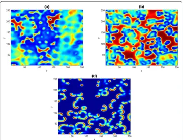
In Fig. 8, we show three typical Turing patterns obtained at (a) ðu^;^vÞ =(11/45, 110/ 253) fort= 300 and (b) ð Þ^u^v =(0.05, 0.062) fort= 500. In both panels, we noticed the formation of Turing spots pattern emanating from the center of the domain, as a result, we fixed the parameter values as in (b) and increase the simulation time to t= 700. A pattern containing the mixture of spots and moon-like stripe patterns emerged in (c). From (a-c) one can observed that irregular patterns prevail in the entire domain. However, the three patterns are essentially different from one another, because of their different wavelengths. We believe the possibility of getting other Turing dynamical structures depending on the choice of initial data and the length of simulation.
0 0.5 1 1.5 2
0 0.2 0.4 0.6 0.8 1 1.2 1.4 1.6 1.8 2
u
v
(a)
f > 0 f < 0
g > 0 g < 0 1 − u −φv=0 1 − v − ψu=0
Stable coexistence
0 0.5 1 1.5 2
0 0.2 0.4 0.6 0.8 1 1.2 1.4 1.6 1.8 2
u
v
(b)
Fig. 6A Lotka-Volterra graph depicting stable equilibrium between two competing species of system (39). Stable coexistence occurs when the isoclines are arranged in (a) forK1<K2/ψandK2<K1/φ. The intersection
point of the two lines gives the positive steady state in (a) where the point (1.4, 1.4) corresponds to (1/φ, 1/
ψ). The locations of the isoclines in (b) indicate that species u out-competes species v and the point (1/
Mutualism system
This is a type of association in theoretical ecology in which the existence of one species has no negative influence on the other. This type of model receives little attention and has not been studied as others, even though its importance is comparable to that of prey-predator and competition models. To start with, we shall analyze briefly the two-species model
∂U ∂T ¼σ1∂
2U
∂X2þF Uð ;VÞ; ∂V
∂T ¼σ2 ∂2V
∂X2þG Uð ;VÞ;
)
ð43Þ
where F(U,V) =α1U(1−U/K1+β1V/K1) and G(U,V) =α2U(1−V/K2+β2U/K2) are the nonlinear reaction terms for the two species U and V, respectively. Andσ1,σ2,α1,α2,β1,
β2,K1,K2are all positive parameters. This system looks similar to equation (36), with exception that β's are treated positive in this case. We then nondimensionalize using the parameters
u tð Þ ¼U Tð Þ K1 ;
v tð Þ ¼V Tð Þ K2 ;
t¼α1T; μ¼αα2 1; φ
¼β2 K2 K1; ψ
¼β1 K1 K2; σ
¼σ2
σ1;
ð44Þ
which on substitution in (43) yields
0 1 2 3 4 5
0.86 0.88 0.9 0.92 0.94 0.96 0.98 1
time
population density
(a)
u v
0 5 10 15 20 25 30 35 40
0.86 0.88 0.9 0.92 0.94 0.96 0.98 1
time
population density
(b)
u v
Intense competing region Coexisting region
0 5 10 15 20 25 30 35 40
0.8 0.82 0.84 0.86 0.88 0.9 0.92 0.94 0.96 0.98 1
time
population density
(c)
u v
0.86 0.88 0.9 0.92 0.94 0.96 0.98 1 0.86
0.88 0.9 0.92 0.94 0.96 0.98 1
Local species u density
Local species v density
(d)
Fig. 7Behaviour of competitive model (38) around the equilibrium states. Declining population density associated with the competitive system is demonstrated in panels (a) and (b). As the resources declined, the two species compete for the limited resources, as evident in panel (b). Parameter values: (a)û=^v=1,
∂u ∂t ¼
∂2u ∂x2þ u−u
2þφuv
¼f uð ;vÞ;
∂v ∂t¼σ
∂2v
∂x2þμ v−v 2þψuv
¼g uð ;vÞ:
)
ð45Þ
Again, by following the linear stability analysis, we study the stability criteria for the non-diffusive system
du
∂t ¼ u−u 2þφuv
¼f uð ;vÞ;
dv
∂t ¼μ v−v2þψuv
¼g uð ;vÞ;
)
ð46Þ
It is not difficult to see that the steady statesðu^;^vÞfor this system are
^ u;^v
ð Þ ¼ð0;0Þ; ð^u;^vÞ ¼ð1;0Þ; ðu^;^vÞ ¼ð0;1Þ; ðu^;^vÞ ¼ 1þφ
1−φψ; 1þψ 1−φψ
: ð47Þ
The Jacobian or community matrix for this system is
B¼ ∂f ∂u
∂f ∂v ∂g ∂u
∂g ∂v
0 B B B @
1 C C C A
^
u;^v
ð Þ
¼ 1−2−uμψþφv −φu
v μð1−2vþψuÞ
^
u;v^
ð Þ: ð
48Þ
Proceeding in a similar manner like those for the previous cases, we can easily show that the points (0, 0), (1, 0) and (0, 1) are all unstable; the point (0, 0) is unstable node while (1, 0) and (0, 1) are the saddle point equilibria, whereas the fourth steady state
Fig. 8Two dimensional results of the competitive model (38). The patterns are obtained with parameters
for 1−φψ> 0 (located in the positive quadrant) is a stable equilibrium. Mutual display of the species is reflected in Fig. 9, panel (a) shows linear behaviour of speciesuand v. Each of the species experienced an unbounded population growth since the existence of one has no effect on the other and their relationship is linear as in (b).
Two dimensional results for model (45)
Following [34], we take the boundary conditions
∂u ∂t ð Þx;y ¼
∂v
∂t ð Þx;y ¼0; ð49Þ
subject to the axi-symmetric initial conditions
u xð ;y;0Þ ¼u^−0:5e −ς2
20 ;
v xð ;y;0Þ ¼^ve −ς2
20 ;
)
ð50Þ
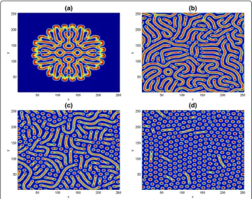
where ς2=x2/2 +y2. We perform some numerical simulations of the dynamical model (45) on the domain size [0, 250] × [0, 250] with time-step Δt= 0.05 and grid width
Δh= 0.5,ð^u;^vÞ=(0.06125, 0.25). We fixed other parameters as in (42) to obtain Fig.10. In the simulations at t= 500, the pattern structures start appearing like a cluster of stripes right from the domain center. It spreads out into irregular stripes as simulation time increased to t= 1000. Later, with further increase in time, the long stripes break into spots at t= 1500 as in (c). In panel (d) at t= 2000, spot patterns have covered the entire domain. Pure Turing spots pattern is achievable if the simulation time is further increased.
In order to justify the suitability and accuracy of the ETDADAMS4 and ETDRK4 schemes, we carried out numerical experiments on the three dynamical systems consid-ered in this paper that is, the prey–predator system (28), competitive system (39), and the mutualism or symbiosis system (45). The performance of ETDRK4 and ETDA-DAMS4 are investigated and compared with the family of exponential time differencing multisteps schemes of order four, five and six which we denoted in this paper for brevity as ETDM4, ETDM5 and ETDM6 respectively.
0 1 2 3 4 5
1 1.02 1.04 1.06 1.08 1.1 1.12 1.14 1.16 1.18
time
population density
(a)
u v
1.05 1.1 1.15 1.2 1.25 1.3 1.35 1.4 1.45 1.5 1.05
1.1 1.15 1.2 1.25 1.3 1.35 1.4 1.45 1.5
Local species u density
Local species v density
(b)
It would go beyond the scope of this paper to give a complete classification of exponen-tial integrators used for comparison. We focus on exponenexponen-tial time differencing method of Adams-type and exponential time differencing Runge-Kutta method, and we have mentioned earlier how they can be treated in the common framework of explicit expo-nential integrators. Details of these schemes are well classified in [16, 41] and references therein, with historical survey offered by Minchev and Wright [30].
We report the maximum relative errors of the solution defined by
relative error¼ max1≤j≤Nu^j−uj
max1≤j≤N u^j
ð51Þ
where û jis a gold-standard run computed with the schemes at Δt= 1/2048 anduj is computed values of the solution u at point j, and N is the number of interior points defined on the collocation interval
x1¼a;…;xi¼aþði−1ÞΔx;…;xN ¼b
f g; Δx¼jb−aj
N−1: ð52Þ
Figure 11 (a) shows the performance of the schemes when applied to the prey-predator system (28) at parameter values t =1, μ= 0.1, ψ= 0.08, φ= 0.01, δ= 0.01 for N= 200. Panel (b) is obtained with parameters t= 1, μ= 0.5, ψ= 0.15, φ= 0.15, δ= 0.5 and N= 200 for the competitive system (39). The performance of the schemes when applied to the mutualism system (45) at parameter values t = 1,
μ= 0.5, ψ= 0.5, φ= 0.5, δ= 0.1, N= 200 is shown in panel (c). We compute the relative errors using a gold-standard run obtained with the schemes using Δt= 1/ 2048 and compare with various time steps 1/2ρ,ρ= 1,…, 10 [34, 36].
It is obvious from the results presented in Fig. 11 that the ETDRK4 has a better convergence when compared to other exponential time differencing methods for each of the problems considered in this paper. Due to the similarity and the choices of parameters used in the simulations of the competitive and the mutualism systems, one observes that the schemes have similar behaviour. The difference is noticeable in their amplitudes. The ETDADAMS4 competes very well with ETDRK4 when applied to the dynamical systems but the ETDRK4 appears to have the overall credit.
The following experiment in Table 1 was performed in one-dimension with predator-prey system (28) in a smaller domain size (0; 100) and the computation was terminated at final time t= 1,…, 4. The parameter values are: μ= 0.4, ψ= 0.08, φ= 0.05, Δt= 0.25 forN= 200. We use the built-in Matlabtic - tocto check the computa-tional time of the schemes. Both schemes runs in seconds. Our numerical experi-ments in one-dimension demonstrate a strong case for abandoning the ETDM4, ETDM5 and ETDM6 schemes. In obtaining the 2D results in Fig. 5, it was observed that the ETDRK4 time-stepping scheme performed about two times faster than the ETDADAMS4 scheme. That is, the computational time required for ETDADAMS4 is about 48 % more than that of the ETDRK4. As a result, we carried out the 2D experi-ments with the ETDRK4 scheme.
10−4
10−3
10−2
10−1
100 10−12
10−10 10−8 10−6 10−4 10−2 100
Time step
Relative errors
(a)
ETDADAMS4 ETDM4 ETDAM5 ETDM6 ETDRK4
10−4
10−3
10−2
10−1
100 10−10
10−9 10−8 10−7 10−6 10−5 10−4 10−3
Time step
Absolute errors
(b)
ETDADAMS4 ETDM4 ETDAM5 ETDM6 ETDRK4
10−4
10−3
10−2
10−1
100 10−10
10−8 10−6 10−4 10−2 100
Time Step
Relative errors
(c)
ETDADAMS4 ETDM4 ETDAM5 ETDM6 ETDRK4
Conclusions
In this paper, firstly, the dynamic complexities of the ecological models consisting of prey-predator, competitive and mutualism reaction-diffusion dynamics are studied by considering their linear stability analysis in the absence of diffusion, and secondly by the numerical approach with the presence of diffusion. We discretized the governing models in space using a fourth-order central finite difference scheme and integrate the resulting ODEs with the exponential time differencing schemes whose formulations were based on the Runge-Kutta and multistep methods of Adams-type. We investigate the stability of the schemes and plots their stability regions. We present the results in both one and two dimensions to unveil their pattern formations. The numerical experi-ments in 2D reveal some of the typical patterns such as stripes and spots, as well as irregular snakelike patterns. Further, we compared the results obtained with both ETDADAMS4 and ETDRK4 for each of the dynamics, with their exponential fourth, fifth and sixth-orders counterparts denoted as ETDM4, ETDM5 and ETDM6, respect-ively, and observed that the ETDRK4 is most reliable and computationally promising in terms of efficiency and accuracy when compared to other methods used in this paper. It worth mentioning that the methodology presented in this work can be extended to higher dimensional practical problems.
Abbreviations
ETDRK4:Fourth-order exponential time differencing Runge-Kutta method; ETDM: Exponential time differencing multistep method; ETDADAMS: Exponential time differencing method of Adams-type.
Competing interests
The authors declare that they have no competing interests.
Authors’contributions
Both OK and PK conceived the research work. Manuscript writing and simulation: OK. Model analysis: OK. Both authors proofread and approved the final manuscript.
Acknowledgements
OK acknowledges the partial financial support from the Federal Government of Nigeria under the 2009 Education Trust Fund Academic Staff Training and Development (AST&D) Intervention. The research contained in this paper is also supported by the South African National Research Foundation (NRF).
Received: 2 October 2015 Accepted: 3 January 2016
References
1. Allee WC. The Social Life of Animals. New York: Norton; 1938.
2. Allen LJS. An Introduction to Mathematical Biology. New Jersey: Pearson Education, Inc.; 2007.
3. Amarasekare P. Interactions between local dynamics and dispersal: insights from single species models. Theor Popul Biol. 1998;53:44–59.
4. Baek H, Jung DI, Wang Z. Pattern formation in a semi-ratio-dependent predator-prey system with diffusion. Discr Dyn Natur Soc. 2013;2013(657286):14. doi:10.1155/2013/657286.
5. Berryman AA. Population Systems: A General Introduction. New York: Plenum Press; 1981.
Table 1The computational time for the ETDRK4 and ETDADAMS4 methods when applied to the
predator-prey system (28) for some values ofδand final timet
Method δ t= 1 t= 2 t= 3 t= 4
ETDRK4 0.25 0.32 s 0.37 s 1.01 s 0.98 s
0.50 1.04 s 0.99 s 1.11 s 1.02 s
1.00 1.15 s 1.32 s 1.88 s 3.87 s
ETDADAMS4 0.25 0.28 s 0.54 s 1.52 s 1.63 s
0.50 1.51 s 1.50s 1.49 s 1.55 s
6. Cox SM, Matthews PC. Exponential time differencing for stiff systems. J Comput Phys. 2002;176:430–55. 7. Dennis B. Allee effects: population growth, critical density, and the chance of extinction. Nat Res Model. 1989;3:481–538. 8. Du Q, Zhu W. Analysis and applications of the exponential time differencing schemes and their contour
integration modifications. BIT Numer Math. 2005;45:307–28.
9. Lopez-Fernandez M, Palencia C. On the numerical inversion of the Laplace transform of certain holomorphic mappings. Appl Numer Math. 2004;51:289–303.
10. Gakkhar S, Naji RK. Order and chaos in s food web consisting of a predator and two independent preys. Commun Nonl Sci Numer Simul. 2005;10:105–20.
11. Garvie M. Finite-difference schemes for reaction-diffusion equations modeling predator-pray interactions in MATLAB. Bullet Math Biol. 2007;69:931–56.
12. Garvie M, Trenchea C. Spatiotemporal dynamics of two generic predator-prey models. J Biol Dyn. 2010;4:559–70. 13. Gyllenberg M, Hemminki J, Tammaru T. Allee effects can both conserve and create spatial heterogeneity
inpopulation densities. Theor Popul Biol. 1999;56:231–42.
14. Harmon JP, Andow DA. Indirect effects between shared prey, predictions for biological control. Biol Control. 2004; 49:605–25.
15. Hochbruck M, Ostermann A. Exponential Runge-Kutta methods for parabolic problems. Appl Numer Math. 2005; 53:323–39.
16. Hochbruck M, Ostermann A. Exponential multistep methods of Adams-type. BIT Numer Math. 2011;51:889–908. 17. Holmes EE, Lewis MA, Banks JE, Veit RR. Partial differential equations: Spatial interactions andpopulation dynamics.
Ecology. 1994;75:17–29.
18. Holt RD. Predation, apparent competition, and the structure of prey communities. Theor Popul Biol. 1977; 12:197–229.
19. de la Hoz F, Vadilo F. An exponential time differencing method for the nonlinear schrodinger equation. Comput Phys Commun. 2008;179:449–56.
20. Janzen DH. The natural history mutualisms. In: Boucher DH, editor. Biol Mutual. Oxford: Oxford University Press; 1985. p. 44–99.
21. Kassam AK, Trefethen LN. Fourth-order time-stepping for stiff PDEs. SIAM J Sci Comput. 2005;26:1214–33. 22. Kawasaki K, Mochizuki A, Matsushita M, Umeda T, Shigesada N. Modeling spatio-temporal patternsgenerated by
Bacillus subtilis. J Theor Biol. 1997;188:177–85.
23. Kot M. Elements of Mathematical Ecology. United Kingdom: Cambridge University Press; 2001. 24. Lotka AJ. The Elements of Physical Biology. Baltimore: Williams and Wilkins; 1925.
25. Lotka AJ. The growth of mixed populations, two species competing for a common food supply. J Washington Acad Sci. 1932;22:461–9.
26. Malchow H. Spatio-temporal pattern formation in nonlinear nonequilibrium plankton dynamics. Proc Roy Soc London B. 1993;251:103–9.
27. Medvinsky AB, Petrovskii SV, Tikhonova IA, Malchow H, Li BL. Spatiotemporal complexity of plankton and fish dynamics. SIAM Rev. 2002;44:311–70.
28. Mendez V, Fedotov S, Horsthemke W. Reaction-Transport Systems: Mesoscopic Foundations, Fronts, and Spatial Instabilities. Berlin Heidelberg: Springer; 2010.
29. Mimura M, Sakaguchi H, Matsushita M. Reaction-diffusion modelling of bacterial colony patterns. Physica A. 2000; 282:283–303.
30. Minchev BV, Wright WM. A review of exponential integrators for first order semi-linear problems, Technical Report NTNU. Department of Mathematical Sciences, Norwegian University of Science and Technology, (2005), Preprint. 31. Murray JD. Mathematical Biology. Berlin: Springer; 1989.
32. Murray JD. Mathematical Biology I: An Introduction. New York: Springer; 2002.
33. Murray JD. Mathematical Biology II: Spatial Models and Biomedical Applications. Berlin: Springer; 2003. 34. Owolabi KM. Robust IMEX schemes for solving two-dimensional reaction-diffusion models. Int J Nonlinear Sci
Numer Simul. 2015;16:271–84.
35. Owolabi KM, Patidar KC. Numerical solution of singular patterns in one-dimensional Gray-Scott-like models. Int J Nonlinear Sci Numer Simul. 2014;15:437–62.
36. Owolabi KM, Patidar KC. Higher-order time-stepping methods for time-dependent reaction-diffusion equations arising in biology. Appl Math Comput. 2014;240:30–50.
37. Petrovskii S, Kawasaki K, Takasu F, Shigesada N. Diffusive waves, dynamic stabilization and spatio-temporal chaos in a community of three competitive species. Japan J Industr Appl Math. 2001;18:459–81.
38. Petrovskii S, Malchow H. Wave of chaos: new mechanism of pattern formation in spatio-temporal population dynamics. Theor Popul Biol. 2001;59:157–74.
39. Petrovskii S, Morozov AY, Venturino E. Allee e_ect makes possible patchy invasion in a predator-prey system. Ecol Lett. 2002;5:345–52.
40. Satnoianu RA, Menzinger M, Maini PK. Turing istabilities in general systems. J Math Biol. 2000;41:493–512. 41. Schmelzer T, Trefethen LN. Evaluating matrix functions for exponential integrators via Caratheodory-Fejer
approximation and contour integrals. Elect Trans Numer Anal. 2007;29:1–18.
42. Sherratt J. Periodic travelling waves in cyclic predator-prey systems. Ecol Lett. 2001;4:30–7. 43. Volpert V, Petrovskii S. Reaction-diffusion waves in biology. Phys Life Rev. 2009;6:267–310.
44. Volterra V. Fluctuation in abundance of the species considered mathematically. Nature. 1926;118:558–60. 45. Volterra V. Variations and Flunctuations of the Numbers of Individuals in Animal and Species Living together,
Reprinted in 1931 in R.N. Chapman, Animal Ecology. New York: McGraw-Hill, 1926.
47. Wang W, Zhang L, Wang H, Li Z. Pattern formation of a predator-prey system with Ivlev-type function response. Ecol Model. 2010;221:131–40.
48. Yu H, Zhong S, Agarwal RP. Mathematics and dynamic analysis of an apparent competition community model with impulsive effect. Math Comput Model. 2010;52:25–36.
49. Yu H, Zhong S, Agarwal RP, Xiong L. Species permanence and dynamical behavior analysis of an impulsively controlled ecological system with distributed time delay. Comput Math Applic. 2010;59:3824–35.
• We accept pre-submission inquiries
• Our selector tool helps you to find the most relevant journal
• We provide round the clock customer support
• Convenient online submission
• Thorough peer review
• Inclusion in PubMed and all major indexing services
• Maximum visibility for your research
Submit your manuscript at www.biomedcentral.com/submit