Research article
Available online www.ijsrr.org
ISSN: 2279–0543
International Journal of Scientific Research and Reviews
Modelling and Simulation of Multi Automated Guided Vehicles in a
Factory Layout
Srinivas. C*
and Chittaranjan Das. V
Asoociate.Professor, Dept. of Mechanical Engg., R.V.R & J.C.College of Engg., Guntur,India
ABSTRACT
An Automated guided vehicle system (AGV’S) is a material handling system in which computer controlled vehicles move along a guide path carrying loads from pickup and deposit (P&D) stands to other P&D stands as they are directed by the computer. AGV systems are invariably used for material handling in FMS due to their flexibility in various aspects. The paper is about modeling and simulation of a factory layout that may contain a number of manufacturing cells and multiple AGV’S that commute between dynamically determined starting and end nodes. A model of a factory layout is build by Flexsim software and an analysis is done on the model based on various performance measures such as throughput, staytime of AGV’S, average time spent by work-in-process jobs waiting for AGV. By testing various dispatching strategies which define the manner in which the jobs arriving to use an AGV is assigned to a selected job, the best strategy is suggested based on the selected performance measures. Simulation enables more efficient planning of the whole manufacturing process, easy modifications before implementation on the real system. By performing simulation on the model the optimum number of AGV’S for a given layout is found out based on selected performance measures
KEYWORDS:
Modeling, Simulation, AGV system, Dispatching, Optimization.Corresponding Author
-
Srinivas. C
Dept. of Mechanical Engg.,
R.V.R & J.C.College of Engg., Guntur,India
E.Mail – [email protected], [email protected],
1.
INTRODUCTION
Material handling is a system or combination of methods, facilities, labor and storing of
materials to meet specific objectives. The purpose of material handling in a factory is to move raw
materials, work in process, finished parts, tools and supplies from one location to another to facilitate
the overall operations of manufacturing .The handling of materials must be performed safely,
efficiently, in a timely manner, accurately (the right materials in the right quantities to the right
location), and without damage to the materials. The cost of material handling is a significant portion
of the total cost of production1. Estimates of handling cost run as high as two-thirds of the total
manufacturing cost.
The material handling function is also concerned with material storage and material control
.The material control function is concerned with the identification of the various materials in the
handling system, their routings and the scheduling of their moves. In most factory operations, it is
important that the origin, current location, and future destination of materials be known. This control
is sometimes augmented by means of an automatic identification system whose purpose is to identify
parts as they are moved or stored.
A material handling system can encompass as entire plant and in some cases, even the
facilities of suppliers and customers. In manufacturing plant, for example it may begin at the
receiving dock and continue through inspection, storage, processing, packaging and shipping. It can
also include packaging and shipping operations at the supplier’s plan as well as unloading and
handling at the customer site.
Regardless of size and complexity, a material handling system should contain two parallel
flows and physical flow of materials and a corresponding flow of information. The flow of
information indicated below therefore provides the basis for controlling the operations.
There are two types of material handling systems
1. Serial access transport systems (e.g. Conveyor systems)
2. Direct or random access transport systems (e.g. automated guided vehicle systems)
The random access systems are more flexible. They can simplify dynamic scheduling and flexible
control of the system and they can strongly modify the traditional process of FMS
1.1 Automated Guided Vehicle Systems
With the introduction if advanced manufacturing technology, computer Flexible
Manufacturing Systems (FMSs) have taken life and Automated Guided Vehicles (AGVs) are
An automated guided vehicle system is a material handling system in which driverless
computer controlled vehicles move along a guide path carrying loads from pickup and delivery
(p&d) stands to other p&d stands as they are directed by the computer. The vehicles are powered by
means of on-board batteries that allow operation for several hours between recharging3. In present
work, FLEXSIM, a general-purpose simulation package has been used for scheduling and planning
of AGV systems for a factory layout.
1.2 Simulation and Modelling
Simulation means imitating the behaviour of a dynamic system through time in order to solve
a given problem. The model is a simplified representation of this system. It is also created and valid
only for this given problem because it is not possible to create a model of a system in all its
dimensions. During the simulation, observations are only estimates, i.e. results can only be given
with a confidence interval.
Modelling and simulation (M&S) is a problem-solving methodology for analyzing complex
systems 4 defines simulation as “the modelling of a process that mimics the response of the actual
system to events that take place over time”. In addition to this,defines simulation as “the process of
designing a model of a real system and conducting experiments with this model for the purpose of
understanding the behaviour of the system and evaluating various strategies for the operating
system”5. The model can be used to
Analyse current operations and identify problem area, e.g. bottlenecks,
Test various scenarios for improvement,
Design new manufacturing systems.
Simulation models allow to test potential changes in an existing system without disturbing
it or to evaluate the design of a new system without building it6. Simulation early in the design cycle
is important, because the cost to repair mistakes increases dramatically the later in the product life
cycle the error is detected. This methodology also allows comparing new concepts, equipments or
scenarios before purchasing. For some purpose, simulations are better than the analysis of real data.
With real data, it is never possible to perfectly know the real-world process that caused a particular
measured situation, because of the too complex interactions inherent in large systems. In a
simulation, the analyst controls all the factors making up the data and can manipulate them
systematically to see directly how specific problems and assumptions affect the analysis. Because
simulation software keeps track of statistics about model elements, performance can be evaluated by
Business processes such as supply chain, customer service and product development are
nowadays too complex and dynamic to be understood and analysed with spreadsheets or flowchart
techniques. The interactions of resources with processes, products and services result in a very large
number of scenarios and outcomes that are impossible to understand and evaluate without the help of
a computer simulation model. Old techniques are adequate for answering “what” questions, but not
for “how”, “when” and “what if” questions.
1.2.1
Discrete-Event Simulation
Discrete-event modelling and simulation is needed for comparing alternatives in analysing, testing
and design of production systems in presence of randomness. Flexibility of the modelling approach
is important, especially for comparisons of intelligent scheduling policies.
The first aim of simulation is to experiment new methods on a computer model because
simulation is cheaper and faster than real experiments, and sometimes it is simply impossible to do
the same on a real process. Another advantage is that a new method can be tested and validated
without disrupting the real system. Simulation can also be used to create models of non-existent
processes when designing new systems or redesigning and reorganizing existing ones.
Historically, discrete event simulation was a part of operational research. It was used to answer
“what if…” questions in order to evaluate the performance of a system. However, it should be kept
in mind that this role of performance evaluation doesn’t guarantee an optimal solution. Commonly,
simulation is used to compare solutions under some parameters and hypothesis. It is up to the user to
define if randomness has an influence or not on the result of the simulation. Results obtained by
simulations are therefore only observations and a statistical and probabilistic approach is needed to
interpret these results.
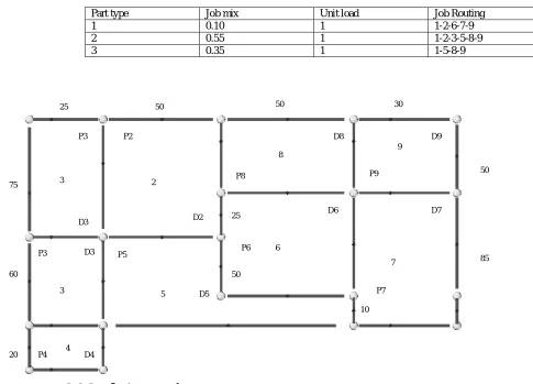
2. SYSTEM DESCRIPTION
The system to be studied is a block layout with a unidirectional loop for the travel of an AGV.
The system is shown in fig 1 below. The system consists of 9 machine centers and 3 types of parts
and the distance between the departments is illustrated in the figure 1. There are 11 control points
and they are represented by Pi and Di where Pi represents the pickup point for department i and Di
represents the delivery point for department i.
The parts flow through the job in the order specified in the production plan. The transfer of
materials across various work centers will be done with the help of AGV’s. Various simulation
strategies will be used to evaluate the dispatching rules for the AGV. The AGVs move on a
Table No.1: Part Type and their Routing.
Fig.1 .
Fig 1. Layout of the System
2.1 Study Assumptions
Inter-arrival times are exponential-
We assume a Poisson job arrival rate and hence an exponential inter-arrival time so that our
system remains at par with a real time situation. The inter-arrival times are in exponential
distribution. Any distribution for the arrival of jobs is not going to have any effect on the
performance of a particular dispatching rule being simulated. We thus assume this distribution
since it is most likely to be true and easier to analyze.
Processing times are normal-
The probability distribution assumed for such a system will not have any effect whatsoever on
the final outcome of the simulation, as the objective here is to simulate various dispatching rules.
Moreover, processing times in a system are usually deterministic and their error is normally
distributed. Hence we assume normally distributed processing times.
Loading and unloading times for the load are assumed to be 10 seconds each. These are
commensurate with industry standards.
Part type Job mix Unit load Job Routing
1 0.10 1 1-2-6-7-9
2 0.55 1 1-2-3-5-8-9
3 0.35 1 1-5-8-9
25 50 P5 D5 5 P6 D6 6 50 P2 D2 2 50 P8 D8 8 25 60 20 75
P3 D3
3 P3
D3 3
P4 4 D4
Values of processing times have been selected such that they do not act as a bottleneck in the
network. Also, the numbers of AGVs have been decided based on the fact that they too do not
become the bottleneck in the network. Each job constitutes a unit load and mass is conserved
during the network flow. This is a reasonable assumption as in a factory layout as it is possible to
get an AGV design or capacity according to requirements.
The speed specifications of the AGVs are pre-determined. We assume 2 feet/minute. It is
possible to change the speed using the AGV controls.
There are 11 control points on the AGV route. The AGV can be stopped at any control point and
only at a control point. Most of these control points are designated pickup and delivery stations,
while others have been designed to park idle AGVs in the network. When an AGV is blocked by
another AGV right in front of it, the AGV in front can be moved to a control point to facilitate
smooth movement of the AGVs in the network.
The above study assumptions also cover our input data. These assumptions and data are based
on prior research that has been carried out in this field. It is important to mention here, that some of
the data are deterministic, while some are stochastic.
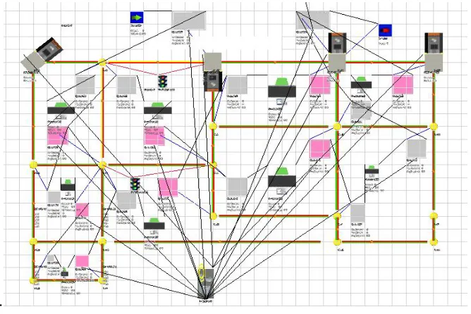
3. BUILDING THE MODEL
First the model of the layout is created using Flexsim software The factory layout is created
as shown below and by clicking and dragging from the object library the objects such as queue, sink,
source, processor, AGV, dispatcher, traffic controller etc. the model is created. After building the
whole layout make connections for each queue so that different types of parts follow different routes
.
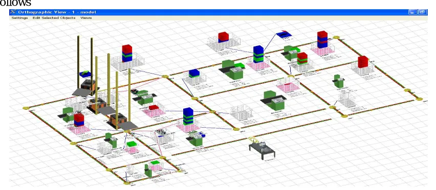
After building the system, the factory layout we compile, reset and run we get the simulation as follows
Fig 3 Factory layout model after simulation is performed
4. THE VARIOUS DISPATCHING STRATEGIES THAT ARE USED FOR
SIMULATION ARE
1. Pass to first available object. If there are none currently available than queue the task
sequence up using the queue strategy and wait until someone connected to its output ports
becomes available.
2. Shortest distance strategy: Pass to the object that is closest to the destination (if the object is
on a network, then network travel is calculated; otherwise centroid to centroid distance is
used).If true then only consider objects which are not busy. In such a case, if none are found
then the task sequence will be queued up using the queue strategy and will be sent to first
available port.
3. Shortest queue strategy: Pass to the object whose task sequence queue is shortest.
4. Round robin strategy: Used to evenly distribute the task sequences among all the task
executes connected to output ports on the current object.
Table No. 2: Throughput for different dispatching strategies
Type of pattern
THROUGHPUT
1AGV 2AGV’s 3AGV’s 4AGV’s
Round Robin Fashion
5 17 26 30
Pass to first available port
5 14 24 30
Shortest distance strategy
5 14 23 29
Shortest queue strategy
From the above table 2 it can be concluded that dispatching strategy round robin fashion
strategy is the better one. Fig 2 shows the model build by using Flexsim of the system and Fig 3
depicts the model during simulation.
5. PERFORMANCE EVALUATION OF AGV SYSTEM
Performance evaluation of AGV for a flexible manufacturing system involves in knowing
the utilization of the various AGVS present in the system .It is also concerned with finding out the
total work station wait time and total AGV wait time. The design modifications to the AGV track can
also be carried out if the standard reports are available. One of the critical factor that helps in
determining the optimum number of AGV’s in a given layout is the throughput and other factors like
total stay time of the queue etc..
More over the behaviour of the AGV system in general can be studied in detail by looking at
the animated movements of the AGVs present in the system on the computer screen.
6. RESULTS
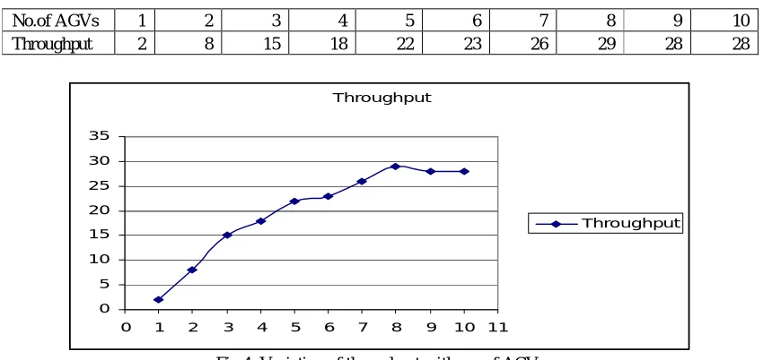
The optimal no of AGV’s for the path is found out by drawing graphs between throughput
and no of AGV’s for the output queue is as follows.Table3,4,5 gives the how through put, stay time
of the system gets effected with the change in the number of AGVs.
Table 3: Variation of throughput with no of AGVs:
No.of AGVs 1 2 3 4 5 6 7 8 9 10
Throughput 2 8 15 18 22 23 26 29 28 28
Fig 4: Variation of throughput with no. of AGVs
Table No. 4: Variation of stay time at final out put queue with number of AGVs
No.of AGVs
1 2 3 4 5 6 7 8 9 10
Stay time 612.5 380.44 316.61 308.69 270 261 247 231.5 227 225 Throughput
0 5 10 15 20 25 30 35
0 1 2 3 4 5 6 7 8 9 10 11
Fig 5: Variation of stay time with no of AGVs
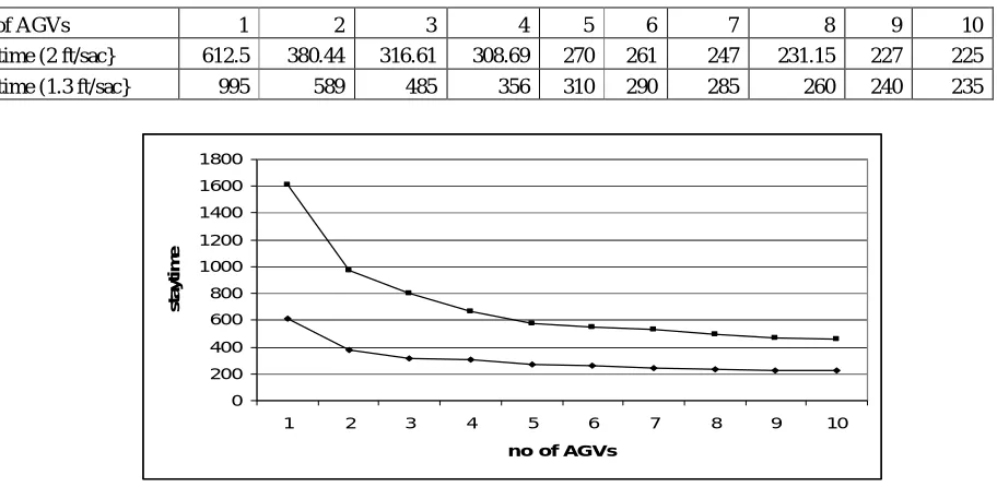
Table No.5: Variation of Stay time of AGV’s for two speeds:
No. of AGVs 1 2 3 4 5 6 7 8 9 10
stay time (2 ft/sac} 612.5 380.44 316.61 308.69 270 261 247 231.15 227 225 stay time (1.3 ft/sac} 995 589 485 356 310 290 285 260 240 235
Fig 6: Variation of stay time for different speeds of AGV’S
From the above figures, Fig 4, Fig 5 and Fig 6 it can be observed that throughput increases
for the given factory layout as the AGV’S increases and this happens up to AGV’S number reach
eight after which even an increase in AGV’S does not contribute to increase in throughput. Similarly
stay time of the items in queue decreases as the number of AGV’S increases up to eight after that the
stay time almost remains constant .Hence it can be concluded that the optimum number of AGV’S in
the given factory layout is eight.
stay
0 100 200 300 400 500 600 700
0 1 2 3 4 5 6 7 8 9 10 11
stay
0 200 400 600 800 1000 1200 1400 1600 1800
1 2 3 4 5 6 7 8 9 10
no of AGVs
s
ta
y
ti
m
7. CONCLUSION
In summary, this paper involves developing the model, simulating the dispatching strategies
for one and more than one AGVs in a unidirectional block layout involving 11 control points. One of
the most important point we have found from this simulation is that for a single AGV and the given
block layout, it does not matter whatever dispatching or service strategies are used and they yield the
same result. For two, three and four AGV’s, round robin strategy is suitable. By selecting the round
robin strategy and simulating the system and selecting the criteria for performance evaluation as the
throughput and stay time the optimum number of AGV’s was found out to be 8 for the given layout.
7.1 Scope of Future work
After doing this project, we feel that the following points will be interesting topics for future study in
this area:
1. One of the interesting points for future research is to evaluate the performance of an AGVs given
that a scheduling system is in place that schedules the jobs to machines according to some
criteria. One method of doing that is to build a model that incorporates this scheduling system
and then inserting the AGVs into the system dispatching them according to the dispatching rules.
We feel this would more realistically represent the system under consideration.
2. The second point of future research is to study the effect of blocking when more than one AGV is
involved in greater detail.
REFERENCES
1. Tompkins J.A, White J.A, Bozer Y.A, Tanchoco J.M.A .Facilities planning. Wiley, New
Jersey. 2003.
2. Kasilingam R.G, Mathematical modeling of the AGVs capacity requirements planning
problem. Eng Costs Prod Econ .1991; 21: 171–175
3. Egbelu P.J . Concurrent specification of unit load sizes and automated guided vehicle
fleet size in manufacturing system. Int Journal Prod Econ. 1993; 29; 49–64
4. Banks.J, Carson J.S, Nelson B.L. Discrete-Event System Simulation, Prentice Hall Inc.
1995.
5. Pegden C.D., 1992. Shannon R.E., Sadowski R.P. Introduction to Simulation Using
SIMAN, McGraw-Hill Inc. 1990.
6. Pidd M. Computer Simulation in Management Science, John Wiley & Sons Ltd.1998.
7. Tang L.L, Yih Y, Liu C.Y. A study on decision rules of a scheduling model in an FMS.
8. Lee J, Roo-Con Choi R, Khaksar M. Evaluation of automated guided vehicle systems by
simulation. Computers and Industrial Engineering. 1990; 19 : 318-21.
9. Vosniakos G.C, Mamalis A.G. Automated guided vehicle system design for FMS
applications. International Journal of Machine Tool Manufacture. 1990; 30: 85-97.
10.Groveer, M.P. Automation, Production Systems and computer Aided Manufacturing,
Prentice Hall Inc. Englewood Cliffs, N.J. 1980.
11.Vis F. A.Survey of research in the design and control of automated guided vehicle
systems, European Journal of Operational Research. 2006 ; 170: 677 -709.
12.Nishi .T and Maeno R. Petri Net Decomposition Approach to Optimization of Route
Planning Problems for AGV Systems, Automation Science and Engineering, IEEE
Transactions on, 2010;7: 523 -537.
13.Liu Y., Gu Y., and Chen J. A New Control Structure Model Based on Object-oriented