Damping Estimation In Thin Walled Structures Using Finite Element Analysis

(1)

IJEDR1602220

International Journal of Engineering Development and Research (www.ijedr.org)

1246

Damping Estimation In Thin Walled Structures Using

Finite Element Analysis

1_{B Anil Kumar,}2_{B Murali Krishna,} 3_{A Purender Reddy} 1_{Assistant Professor,}2_{Assistant Professor,} 3_{Assistant Professor}

Department of Mechanical Engineering,

1_{Princeton college of engineering & Technology,}2_{Princeton college of engineering & Technology,}3_{Sphoorthy Engineering} college, Hyderabad, India

________________________________________________________________________________________________________ Abstract - By performing modal analysis by finite element analysis gives us only natural frequencies and mode shapes, but not modal damping ratio values. To obtain the modal damping ratio values establishment of a constitutive relation for specific material dissipation, volume integrals of the per cycle dissipation can be used to estimate the modal damping ratios. Here, a well-known power law model for such specific dissipation is used. The development of a modal damping estimation procedure for thin-walled components using shell elements in a commercial finite element package is made. The validation of the shell element results are compared with analytical results and both the results turns out to be same. The computational approach allows complex geometries in a study of the effects of shape on damping. Then demonstration of both the stress concentrations and small tuned resonant appendages yields in increasing damping. Various thin walled structures are taken and the damping values are calculated.

Index Terms: Finite Element Analysis (FEA), Damping, Modal Analysis.

________________________________________________________________________________________________________

I.INTRODUCTION

Computational procedure for the modal damping ratios of engineering components will give us better results rather than guessing. For two things are to be established here (i) a relation for specific material dissipation i.e., energy dissipation within the material per cycle of stress and per unit volume and (ii) a computational relation using such a constitutive relation to find a dissipation for an object vibrating in its first natural modes. Development of a computational procedure for thin-walled structures by using the shell elements in finite element package. The reason for using shell elements is that components which are thin walled gives fast results rather than the solid element results. Firstly we take a thin plate rectangular plate, then a square plate, then a square plate with slots, then a rectangular plate, then a rectangular plate with small appendages and a shell.

Thin-walled structures comprises an important and growing proportion of engineering construction with areas of application becoming increasingly diverse, ranging from aircraft, bridges, ships and oil rigs to storage vessels, industrial buildings and warehouses. Many factors, including cost and weight economy, new materials and processes and the growth of powerful methods of analysis have contributed to this growth, and led to the need for a journal which concentrates specifically on structures in which problems arise due to the thinness of the walls. This field includes cold– formed sections, plate and shell structures, reinforced plastics structures and aluminum structures, and is of importance in many branches of engineering .The primary criterion for consideration of papers in Thin–Walled Structures is that they must be concerned with thin–walled structures or the basic problems inherent in thin–walled structures. Provided this criterion is satisfied no restriction is placed on the type of construction, material or field of application.

II.OBJECTIVES

The objectives of the present work are follows:

 To determine the modal damping ratio by the extraction of stresses and by performing the modal analysis by using Femap software. Calculating the damping ratios analytically for simply supported rectangular plate with the help of the Kirchhoff’s plate theory. Then comparing the damping ratios analytically result with the analysis work

 To find the damping values for the square plate with and without slots and compare the values obtained between them by performing free-free modal analysis.

 To determine the damping values for a rectangular plate with and without appendages and compare the values obtained between them by performing free-free modal analysis.

III.LITERATURE REVIEW

(2)

IJEDR1602220

1247

implementation on commercial structures has taken place very quickly. With specific case studies for four of the more than 300 major buildings and bridges equipped with fluid dampers by Taylor Devices, Inc., a defence contractor from the Cold War years. D. Taylor [2] given The Application of Energy Dissipating Damping Devices to an Engineered Structure or Mechanism. The design of a structure or mechanism subjected to shock and vibration can be greatly improved by the addition of isolation or damping devices. Improvements Include: Reduced Deflection and Stresses, Reduced Weight, Improved Bio dynamics, Longer Fatigue Life, Architectural Enhancement and Reduced Cost.

D. Lee and D. Taylor [3] said that viscous dampers can protect structures against wind excitation, blast and earthquakes. Viscous damper technology originated with military and aerospace applications. Approximately 20 years ago it was found that the same fluid viscous dampers that protect missiles against nuclear attack and guard submarines against near miss underwater explosions could also protect buildings, bridges and other structures from destructive shock and vibration.

D. Taylor [4] had given the advent of high speed equipment and machinery has brought with it numerous problems associated with slowing and stopping masses of various forms. The hydraulic shock absorber has proven to be one of the most satisfactory means of solving these problems, yet the shock absorber still remains as one of the least understood fluid power components. He gives information about the presents design constraints, design parameters and a description of how to use shock absorbers into a system for the purpose of dissipating kinetic energy. IT is presented in both qualitative and functional equation format to enable the reader to grasp the subjective aspects of shock absorber usage which go beyond normal mathematical constraints.

Gordon R. Johnson [5] had given that a series of parametric studies have been presented on investigating the effects of internal soil damping, Poisson’s ratio, layer depth, and embedment on the stiffness functions of circular footings subjected to dynamic forces. The effect of having a finite layer of soil on rigid rock is to introduce valleys in the stiffness’s at the resonant frequencies of the stratum. These valleys are smoothed by the presence of internal damping and their position depends on the value of Poisson’s ratio. Embedded foundations have an increased static stiffness, but the frequency variations of the stiffness coefficients are not very different from the corresponding curve for surface footings. The most important factor in reproducing adequately the effect of embedment is the evaluation of the static stiffness’s. They are, however, very sensitive to the assumed conditions at the vertical edges (sidewalls welded to the surrounding soil, degree of disturbance of the backfill, etc.). Experimental work to assess these conditions is necessary.

IV.FINITE ELEMENT ANALYSIS

Introduction to Modal Analysis:

Modal analysis is an important analysis tool for determining the modal frequencies and shapes of multi-degree freedom of systems. In modal analysis, system is considered to be un damped, as the influence of damping on natural frequency is negligible and the body is executing free vibrations i.e., the system is given some energy in the form of initial displacements or initial velocities or both and it vibrates indefinitely because there is no dissipation of energy. Solution of the equation can be assumed of the form

𝑥𝑖(𝑡) = 𝑋𝑖T (t) i = 1, 2…n (n = Number of degrees of freedom) Equation 3.12

Where 𝑋jis a constant and T is a function of time (t), Equation 3.1 shows that the amplification ration of two coordinates { 𝑥_𝑗(t)

𝑥𝑗(t)}is independent of time. Physically this means that all coordinates have synchronous motions. The configure ration of the system does not change its shape during motion, but its amplitude does. The configure ration of the system, given by the vector

𝑋⃗ =

{ 𝑋1 𝑋_.2

.. . 𝑋𝑛}

Is known as mode shape of the system, which indicates the particular geometrical shape in which the system vibrates at specific natural frequency. Substituting Equation 3.1 in Equation 3.11 results in

[𝑚]𝑋⃗ 𝑇̈(𝑡) + [𝑘] 𝑋⃗⃗⃗⃗ 𝑇(𝑡) = 0⃗⃗ Equation 3.13

Equation 3.2 can be written in scalar form as n separate equations

(∑ 𝑚𝑖𝑗 𝑛 𝑗=1 𝑋𝑗) 𝑇̈(𝑡) + (∑ 𝑘𝑖𝑗 𝑛 𝑗=1

𝑋𝑗) 𝑇(𝑡) = 0, 𝑖 = 1,2,3, … . 𝑛

From which the following relation can be written −𝑇̈(𝑡)

𝑇(𝑡)=

(∑𝑛𝑗=1𝑘𝑖𝑗𝑋𝑗) (∑𝑛𝑗=1𝑚𝑖𝑗𝑋𝑗)

, 𝑖 = 1,2, . . , 𝑛

Since the left side of Equation 3.4 is independent of the index i , and the right side is independent of t, both sides must be equal to a constant. By assuming this constant as 𝜔2_{, we can write eqn (3.4) as}

𝑇̈(𝑡) + 𝜔2_{𝑇(𝑡) = 0} ∑𝑛 (𝑘𝑖𝑗− 𝜔2_{𝑚𝑖𝑗)}

𝑗=1 𝑋𝑗=0,

[[𝑘] − 𝜔2_{[𝑚]]𝑋⃗ = 0}_⃗⃗ _{Equation 3.14}

Solution for the eqn (3.5) can be expressed as

(3)

IJEDR1602220

1248

Where C1 and ∅ are constants, known as the amplitude and phase angle respectively. Equation 3.6 shows that all the coordinates can perform a harmonic motion with the same frequency 𝜔 and the same phase angle∅. However the frequency 𝜔 cannot take any arbitrary value; it has to satisfy the Equation 3.5. Since Equation 3.5 represents a set of n linear homogeneous equations in the unknowns Xi (i=1, 2, 3…, n), the trivial solution is X1 = X2 = … = Xn = 0. For a nontrivial solution equation 3.5, the determinant ∆ or the coefficient matrix must be zero. That is

∆= |kij- 𝜔2𝑚IJ | [k] - 𝜔2 [𝑚]| Equation 3.16

Equation 3.5 represents what is known as the Eigen value or characteristic value, Equation 3.15 is called characteristic equation, 𝜔2_{is known as the Eigen value or characteristic value, and 𝜔is called the natural frequency of the system.}

The expansion of equation (3.16) leads to an nth _{order polynomial equation in 𝜔}2 _{.the solution of this polynomial or characteristic} equation gives n values of 𝜔2_{. It can be shown that al the n roots are real and positive when the matrices [k] and [m] are} symmetric and positive definite. If 𝜔2

1, 𝜔22, ……, 𝜔2n denote the n roots in ascending order of magnitude, their positive square roots give the n natural frequency of the system 𝜔1 ≤ 𝜔2 ≤………..≤ 𝜔n. the lowest value (𝜔1) is called the fundamental or first natural frequency. In general, all the natural frequencies 𝜔i are distinct, although in some cases two natural frequencies might posses the same value.

Several methods are available to solve an Eigen value problem. An elementary method is given below: Equation 3.15 can also be expressed as

[𝜆[k] – [m]] 𝑋⃗ = 0⃗⃗ Where

𝜆 = 1

𝑤2 Equation 3.18

By pre-multiplying equation (3.7) by [k]-1_{, we obtain}

[𝜆[I] – [D]] 𝑋⃗ = 0⃗⃗

𝜆 [I] 𝑋⃗ = [D]] 𝑋⃗ Equation 3.19

Where [I] is the identity matrix and

[D] = [k]-1 _[m]

Is called dynamical matrix. The Eigen value problem of equation 3.19 is known as standard Eigen value problem. For a nontrivial solution of 𝑋⃗⃗⃗⃗, the characteristic determinant be zero i.e,

∆ = | 𝜆 [I] – [D]| = 0 Equation 3.20

On expansion equation (3.20) gives a 𝑛th_{degree polynomial in𝜆, known as characteristic or frequency equation. If the degree of} freedom of the system (𝑛) is large, the solution of this polynomial equation becomes quite tedious.

Once the objectives of the modal analysis have been established, the practical details must be considered. The number and the placement of the exciters should be chosen so that all the modes of interest are excited properly. Similarly, the choice of response measurement locations should allow unique geometrical description of the mode shapes, avoiding problems of spatial aliasing.

V.RESULTS AND DISCUSSIONS

Introduction:

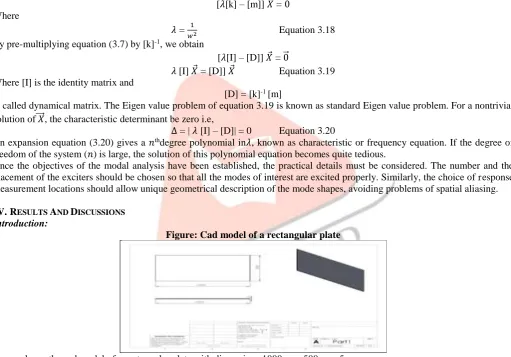
Figure: Cad model of a rectangular plate

Figure shows the cad model of a rectangular plate with dimensions 1000mm×500mm×5mm

Modal damping ratios are calculated for thin walled structures. Modal damping ratios are calculated for a rectangular plate with simply supported boundary conditions and the result is verified with the analytical approach. Then different thin walled structures are taken as examples and the modal damping ratios are calculated and these results are compared with different boundary conditions. The values of the modal damping ratios are found out at obtained natural frequencies.

Table: Properties table for steel

MATERIAL STEEL

YOUNGS MODULUS ( E IN GPA) 210

POISSIONS RATIO 0.3

DESITY (𝜌 in kg/𝑚3₎ ₇₈₀₀

Table shows the necessary material properties of the geometries taken.

Analysis of a Rectangular Plate with Simply Supported Boundary Condition:

(4)

IJEDR1602220

1249

Figure shows the second mode shape of a simply supported rectangular plate and the frequency obtained is 61.53Hz. The numbers of elements are 5000. The numbers of nodes are 35753 and the volume of all the elements is 0.0025𝑚3_{. The average value of} 2𝜋𝜉_𝑒𝑓𝑓

𝐽𝐸 obtained is 0.8681.

Table: Top middle and bottom value of damping for simply supported rectangular plate Top value of

2𝜋𝜉𝑒𝑓𝑓 𝐽𝐸

Middle value of 2𝜋𝜉𝑒𝑓𝑓

𝐽𝐸

Bottom value of 2𝜋𝜉𝑒𝑓𝑓

𝐽𝐸

Average value of 2𝜋𝜉𝑒𝑓𝑓

𝐽𝐸

1.30215 0 1.30215 0.8681

Table gives the information about the top middle, bottom and the Average value of 2𝜋𝜉𝑒𝑓𝑓 𝐽𝐸 Analysis of A Square Plate without Slots with Free-Free Boundary Condition:

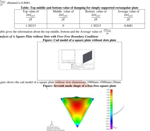
Figure: Cad model of a square plate without slots plate

Figure shows the cad model of a square plate without slots dimensions 1000mm×1000mm×20mm Figure: Seventh mode shape of a free-free square plate

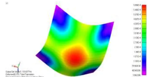
Figure shows seventh mode shape of a free-free square plate without slots and the frequency obtained is 65.2083Hz. The numbers of elements are 400. The numbers of nodes are 1281 and the volume of all the elements is 0.02 𝑚3_{. The average value of}2𝜋𝜉𝑒𝑓𝑓

Figure: Eighth mode shape of a free-free square plate

Figure shows eight modes shape of a free-free square plate without slots and the frequency obtained is 95.306Hz the numbers of elements are 400. The numbers of nodes are 1281 and the volume of all the elements is 0.02𝑚3_{. The average value of}2𝜋𝜉𝑒𝑓𝑓

(5)

IJEDR1602220

1250

Figure shows ninth mode shape of a free-free square plate without slots and the frequency obtained is 118.077Hz. The numbers of elements are 400. The numbers of nodes are 1281 and the volume of all the elements is 0.02𝑚3_{. The average value of}2𝜋𝜉𝑒𝑓𝑓

Analysis of A Square Plate with Slots with Free-Free Boundary Condition:

Figure: Cad model of a square plate with slots

Figure shows the cad model of a rectangular plate with dimensions 650mm×650mm×20mm and slots dimensions are 125mm×50mm.

Figure: Seventh mode shape of a free-free square plate with slots

Figure shows the seventh mode shape of a free-free square plate with slots and the frequency obtained is 66.87Hz. The numbers of elements are 6016. The numbers of nodes are 6273 and the volume of all the elements is 0.20492𝑚3_{. The average value of} 2𝜋𝜉_𝑒𝑓𝑓

(6)

IJEDR1602220

1251

Figure shows the eight mode shape of a free-free square plate with slots and the frequency obtained is 104Hz. The numbers of elements are 6016. The numbers of nodes are 6273 and the volume of all the elements is 0.20492𝑚3_{. The average value of}2𝜋𝜉𝑒𝑓𝑓

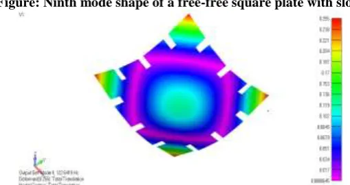
Figure: Ninth mode shape of a free-free square plate with slots

Figure shows the ninth mode shape of a free-free square plate with slots and the frequency obtained is 122.64Hz. . The numbers of elements are 6016. The numbers of nodes are 6273 and the volume of all the elements is 0.20492𝑚3_{. The average value of} 2𝜋𝜉𝑒𝑓𝑓

Table: Results table for a square plate with and without slots.

Mode number Frequency for uncut plate in HZ

Frequency for slotted plate IN

HZ

Average value of 2𝜋𝜉_𝑒𝑓𝑓

𝐽𝐸 for uncut plate

𝐽𝐸 for slotted plate

7 65.2083 66.87 1.0632 1.09

8 95.306 104 1.0391 1.0826

9 118.083 122.64 0.8073 0.8137

Table 5.3 gives the information of average values of 2𝜋𝜉𝑒𝑓𝑓

𝐽𝐸 for free-free boundary condition square plate with and without slots. The values of frequency are increasing from mode 7 to mode 9 and the value of 2𝜋𝜉𝑒𝑓𝑓

𝐽𝐸 from mode 7 mode 9 there is decreasing. At all the particular modes the frequencies and the value of 2𝜋𝜉𝑒𝑓𝑓

𝐽𝐸 are more for a slotted plate when compared with the plate without slots.

Analysis of a Rectangular Plate without Appendages with Free-Free Boundary Condition: Figure: Cad model of a rectangular plate without appendages.

(7)

IJEDR1602220

1252

Figure 5.12 shows the seventh mode shape of a free-free rectangular plate without appendages and the frequency obtained is 52.22Hz. The numbers of elements are 1500. The numbers of nodes are 1581 and the volume of all the elements is 0.006𝑚3_{. The} average value of 2𝜋𝜉𝑒𝑓𝑓

Figure: Eight mode shape of a free-free rectangular plate without appendages

Figure 5.13 shows the eight modes shape of a free-free rectangular plate without appendages and the frequency obtained is 54.01Hz. The numbers of elements are 1500. The numbers of nodes are 1581 and the volume of all the elements is 0.006𝑚3_{. The} average value of 2𝜋𝜉𝑒𝑓𝑓

𝐽𝐸 obtained is1.011

Figure: Ninth mode shape of a free-free rectangular plate without appendages

Figure 5.14 shows the ninth mode shape of a free-free rectangular plate without appendages and the frequency obtained is 122.00Hz. The numbers of elements are 1500. The numbers of nodes are 1581 and the volume of all the elements is 0.006𝑚3_. The average value of 2𝜋𝜉𝑒𝑓𝑓

Figure: Tenth mode shape of a free-free rectangular plate without appendages

Figure 5.15 shows the tenth mode shape of a free-free rectangular plate without appendages and the frequency obtained is 143.739Hz. The numbers of elements are 1500. The numbers of nodes are 1581 and the volume of all the elements is 0.006𝑚3_. The average value of 2𝜋𝜉𝑒𝑓𝑓

(8)

IJEDR1602220

1253

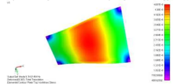
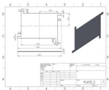
Figure 5.16 shows the cad model of a free-free rectangular plate with appendages with dimensions 1000mm×600mm×10mm and with appendages dimensions 100mm×50mm

Figure: Seventh mode shape of a free-free rectangular plate with appendages

Figure 5.17 shows the seventh mode shape of a free-free rectangular plate with appendages and the frequency obtained is 49Hz. The numbers of elements are 2269. The numbers of nodes are 7058 and the volume of all the elements is 0.0052𝑚3_{. The average} value of 2𝜋𝜉𝑒𝑓𝑓

Figure: Eight mode shape of a free-free rectangular plate with appendages

Figure 5.18 shows the eight modes shape of a free-free rectangular plate with appendages and the frequency obtained is 56.98 Hz. The numbers of elements are 2269. The numbers of nodes are 7058 and the volume of all the elements is 0.0052𝑚3_{. The average} value of 2𝜋𝜉𝑒𝑓𝑓

(9)

IJEDR1602220

1254

Figure 5.19 shows the ninth mode shape of a free-free rectangular plate with appendages and the frequency obtained is 120.45Hz. The numbers of elements are 2269. The numbers of nodes are 7058 and the volume of all the elements is 0.0052𝑚3_{. The average} value of 2𝜋𝜉𝑒𝑓𝑓

Figure: Tenth mode shape of a free-free rectangular plate with appendages

Figure 5.19 shows the eight modes shape of a free-free rectangular plate with appendages and the frequency obtained is 136.2Hz. The numbers of elements are 2269. The numbers of nodes are 7058 and the volume of all the elements is 0.0052𝑚3_{. The average} value of 2𝜋𝜉𝑒𝑓𝑓

Table: Results table for a rectangular plate with and without appendages.

Mode Frequency of a

rectangular plate without appendages

Frequency of a rectangular plate with

appendages

𝐽𝐸 for plate without appendages

𝐽𝐸 for plate with appendages

7 52.22hz 49hz 0.9407 0.988

8 54.01hz 56.98hz 1.011 1.135

9 122.50hz 120.45hz 1.0282 1.088

10 143.739hz 136.20hz 0.945 0.94

Table 5.4 gives the information of average values of 2𝜋𝜉𝑒𝑓𝑓

𝐽𝐸 for free-free boundary condition rectangular plate with and without appendages. From mode 7 to mode 8 he values of the frequencies and 2𝜋𝜉𝑒𝑓𝑓

𝐽𝐸 are increasing but at the tenth mode there is a decrease in the value of 2𝜋𝜉𝑒𝑓𝑓

𝐽𝐸 for both the plate. The plate with appendages requires more amount of damping when compared with plate without appendages.

VI.CONCLUSIONS

If damping value for different structures is calculated before it practical use if offers great savings .There would be no material damage. Many structures tend to vibrate due to forces exerted on it . If we determine the damping value by calculations by applying the necessary boundary conditions ,It would be helpful to select the right geometry and material for that particular boundary conditions and for that particular forces rather than going for experimental testing’s.

 The estimated damping value for a rectangular plate with simply supported boundary condition by analytical approach i.e. 2𝜋𝜉𝑒𝑓𝑓

𝐽𝐸 = 0.8681  The value of 2𝜋𝜉𝑒𝑓𝑓

𝐽𝐸 for a rectangular plate with simply supported boundary condition by performing modal analysis at its first natural frequency 61.53 Hz is 0.8681. Both the analytical and the analysis results turn out to be same.

(10)

IJEDR1602220

1255

 At all the particular modes the frequencies and the value of 2𝜋𝜉𝑒𝑓𝑓

𝐽𝐸 are more for a slotted plate when compared with the plate without slots. The highest amount of damping is for a square plate without slots at the frequency 66.87 Hz is 1.09.  The value of damping can be improved by adding appendages i.e. extra material. The appendages act as vibration

absorbers.

 The plate with appendages with free- free boundary condition requires higher amount of damping than the plate without appendages. The frequencies are increasing from mode 7 to mode 10 and the values of 2𝜋𝜉𝑒𝑓𝑓

𝐽𝐸 are increasing from mode 7 to 9 and there is a decrease at mode 10. The highest amount of damping is for a rectangular plate with appendages at frequency 56.98 Hz is 1.135.

VII.REFERENCES

[1]. R.J.HOOKER Equivalent stresses for representing damping in combined stresses –journal of sound and vibration.

[2]. P. Jana, A.Chatarjee Computational predication of modal damping ratios in thin walled structures –journal of sound and vibration.

[3]. Mechanical vibrations by Grover.

[4]. CONCEPTS AND APPLICATIONS OF FINITE ELEMENT ANALYSIS, 4TH EDITION By Robert D. Cook, Malkus, Plesha, Witt

[5].Solid Works 2015 Part I - Basic Tools, Part 1 By Paul Tran [6]. Finite Element Analysis Concepts: Via Solid Works By J. E. Akin

[7] P. JANA, A.CHATARJEE Computational predication of modal damping ratios in Thin walled structures –journal of sound and vibration

[8] B.J.LAZAN, Damping of materials and members in structural mechanics. [9] A.L. KIMBAL, D.E.LOVELL, Internal friction in solids.