A Perishable Inventory Model with Allowable
Shortages and the Delay in Payment under the
Effect of Inflation
Jitendra Kumar, Pardeep Kumar Sharma, Sunil Kumar, Amit Kumar Rana
Abstract: The article has been developed with lot size model for the perishable material and the deterioration rate is taken to be time varying. Here we have considered that the retailer is offered with the allowable delay in payment for the smooth running. Shortages occurred and the demand is expected to be exponentially increasing, time dependent. Model is developed under inflationary condition. Mathematical model is presented to formulate the problem and the optimal replenishment policies are derived to find the solution. Ultimately, a numerical investigation is given to illustrate the problem and the sensitivity examination is introduced to see the impact of the different parameters.
Keywords: Trade credit, shortages, deterioration, and inflation.
—————————— ◆ ——————————
I.
INTRODUCTION
In most of the available literature researchers developed their inventory model without considering the deterioration, while in practical situations deterioration occurs for almost every product during the storage period, for example vegetables, fruits, chemical, medicines, and electronic equipments. The earliest model of inventory, incorporating the deteriorating items is in the inventory was made by the Ghare and Schrader in 1963. They developed an economic lot size model for the decaying items with constant demand rate. For more insights concerning decaying things the survey paper of Goyal and Giri (2001) is the best source of information. For a very long period it is expected by the analysts that the retailer disburses the costs of the material to the supplier instantly. But in a real environment it is not always possible to pay the amount immediately. Usually supplier offers his client a grace period for the payment and allows him to settle the account without charging the interest. The phenomenon is known as the trade credit policy. The strategy appeals to the consumer to by the product. The earliest approach it the field of delay in payment, was made by the Goyal, (1985). Thereafter, several researchers have developed their model to extend the Goyal’s (1985) model. Another model was developed by Aggarwal, and Jaggi (1995), he has extended the model of Goyal, (1985) to find the optimal replenishment quantity for the decaying items under the effect of trade credit. The model was developed without shortages and the demand and deterioration rate were considered as constant. Furthermore, Singh and Singh (2009, 2010), Yang and Wee (2006), Benkherouf, (1995) and Singh and Kumar (2010) have also considered the permissible delay in their paper. Kumar and Singh (2012) have explored a stock model with volume adaptability under the effect of inflation. Dem, et al., (2014) researched an EPQ stock control framework with seasonal demand under volume adaptability. Kumar, et al., (2015) have built up an EPQ model with admissible delay in imbursement with preservation technology. Saxena, et al., (2017) contemplated a green supply chain framework with reasonable delay in payment. Yadav, et al., (2019) presented
a store network stock model for deteriorating things with warehouse under inflation. Kumar, et al., (2019) have built up an EPQ stock model for seasonal items. Model was deliberated for the deteriorating things with volume adaptability. In the displayed article we have built up an EOQ model for the decaying things and the deterioration is taken to be time subordinate, while the demand rate is thought to be exponentially expanding with time. Model is created with allowable delay in the payment under inflationary environment. Deficiencies are allowed which is partially backlogged.
Assumption and Notation
The model is planned with the assistance of the accompanying assumptions and notation. Assumptions
1. Retailer is offered with the permissible delay in payment. 2. Shortages are permitted which is assumed to be fully backlogged.
3. Deterioration rate
( )
t
=
t
, where 0<
<<1 is taken into consideration and assumed to be time dependent.4. Demand rate D(t) = aebt where a > 0 and b > 0 is supposed
to be time dependent. Especially, it is considered as an exponentially expanding function of time.
5. Model is developed under inflationary conditions. Notations
O Ordering cost M Delay period D(t) Demand rate
(t) Deterioration rate r rate of inflation Sp Selling priceCp Purchasing cost
h Holding cost Cs Shortage cost
Cd Deterioration cost
Ir Interest charge
Ie Interest earned
C1(t1,T) Total expense for the case I
C2(t1,T) Total expense for the case II
C(t1,T) Total expense.
II. MATHEMATICAL MODELING
The stock behavior of this inventory system is depicted in fig 1. Model starts at time zero and then the inventory depletes because of demand and deterioration until the time t1. After that inventory level depletes to zero and shortage ————————————————
*Correspondence Author
• Jitendra Kumar*, Department of Mathematics, Swami Vivekanand Subharti University, Meerut, UP, India. Email: [email protected]
• Pardeep Kumar Sharma, Department of Mathematics, Swami Vivekanand Subharti University, Meerut, UP, India.
• Sunil Kumar, Department of Mathematics, Swami Vivekanand Subharti University, Meerut, UP, India.
6100 start to occur by the time T.
Fig.1: Behavior of Inventory level for the EOQ system
The deviation of level of inventory can be defined by the following differential equations:
1 1
( )
( ) bt, ( ) 0, 0 dI t
I t I t t t
dt + =
−
ae
= (1)
1 1
( )
, ( ) 0,
bt
dI t
ae I t t t T
dt = − = (2)
The solutions of the above differential equations are as follows
1 1 2 2 1
1 1
2
( ) 1 ( ) ( ) ( ) ,
2
bt bt bt bt bt
a
I t e e t e te t t e
b b b
= + − − − + −
1
0 t t (3) 1
1 ( ) a( bt bt),
I t e e t t T
b
= − , (4)
Let we have, I (0) = Q in equation (3), we have
(
1)
11 1
2
1 1
1 1
2
bt bt
a
Q e e t t
b b b
= + − + −
(5)
The most shortage quantity
( )
a bt1(1 b T t( 1))S I T e e
b
−
= − = − − (6)
Therefore, the total ordering quantity
1 2
1 1
2 2
1
2
bt bT
Q S
a a
t t e e
b b b b b
= +
= − + − + −
(7)
Cost Components Ordering cost = A Procurement cost
p
C
= 2 1
1 1
2 2 1 2
bt bT
p
a a
C t t e e
b b b b b
= − + − + −
Storage cost 1
0 ( )
rt
t
h I t e dt
=
( ) ( )
( )
1 1 1
1 1 1 1
1
2 2
2
1 1
1
2 2 2 3 3
1
1 1
2
1 2 2
2
b r t bt b r t
b r t bt rt rt
bt
ha e e e
b b r r b b r b r
t t e
e e e
t e
b r r r r r r r
+ +
+
= + − − + + − +
− − − − − − −
Shortages cost
(
)
( )
(
)
1
1 1
( )
T
rt S
t
bt bT
b r t rT
s
C e dt
a b e e
C e e
b r b r b r r
I t
+
= −
= + + + −
Deterioration cost
(
)
(
)
(
)
(
)
(
)
(
)
( )(
(
(
)
)
(
)
(
)
(
)
(
)
)
1 3 2
3 3
2 2 2 2 2
1 1
4
3 2 3 2 2
1 1 1
3 4
2 3 2 2
1 1 1
3 2 2
1 1 1
1
0
3 2
2
2 2 6 2
1
2 8 5 2
3 3 1
2 9 8 3 2
( ) ( )
rt dd
bx
b r t
t
C
b b r b r
C a
b b r
e r br t b r t
r
b e r r t rt r t
r b r
b r t rt r t
br r t rt r t
t I t e dt
+ =
+ + +
= −
+
− + − + +
+
+ + − + − +
+
+ + − + − +
+ + − + − +
Possibly, two cases are arising here Case I when
1
t
M
and Case II whent
1
M
behavior of the interest earned is depicted in the figure 2.Case I: t1M. Interest Earned
(
) (
)
(
( ))
1 1
1 1
0 0
1
( ( ) )
1 1
1
t t
bt rt bt rt
p e
b r t p e
S I ae te dt M t ae e dt
S I a M e t
b r b r
+
= + −
= − − +
+ +
Interest paid = NIL
Total cost for case 1 is given by
1( , )1
C t T = 1
T (Ordering Cost + Procurement Cost + Storage
Cost + Deterioration Cost+ Backlogging Cost + Interest paid -Interest earned)
Total Annual Cost S
Q
T
t1 Time Retailer’s
( )
(
)
( ) ( ) ( ) 1 1 11 1 1
1
2
1 1 2 1 1 2
2 2
2
1
( , ) 1
2 1 1 1 bt bT p bt bT
b r t rT
s
b r t bt b r t
b r t
a a
C t T C t t e e
T b b b b b
a b e e
C e e
b r b r b r r
ha e e e
b b r r b b r b r
e b r + + + + = − + − + − + + − + + + + − − + + − + −
(
)
(
)
(
)
(
)
(
)
(
)
( )(
(
(
)
)
1 1 1 1 1 2 1 11 2 2 3 3
3 2
3 3
2 2 2 2 2
1 1
4
3 2 3 2 2
1 1 1
3 4
2 3 2 2
1 1 1
2
1 2 2
2
3 2
2
2 2 6 2
1
2 8 5 2
3 3 1
rt
bt rt
bt
d
bx
b r t
t t e
e e
t e
r r r r r r
b b r b r
C a
b b r
e r br t b r t
r
b e r r t rt r t
r b r
b r t rt r t
+ − − − − − − + + + + − + − + − + + + + + − + − + + +
(
+ − +(
− +)
)
(
)
(
)
(
) (
)
(
( )1)
3 2 2
1 1 1
1
2 9 8 3 2
1 1
1 b r t
p e
br r t rt r t
S I a M e t
b r b r
+ + + − + − + − − − + + + (8) From equation (8) it is observed that the total annual cost is the function of the two variables t1 and T. hence to minimize
the total annual cost, we have to differentiate the cost with respect to t1 and T and equating them to zero, we get,
1 1 1 1
1
( , ) ( , ) 0 and 0
C t T C t T
t T
= =
(9)
Satisfying the following conditions
2 2
1 1 1 1
2 2
1
( , ) ( , )
0, 0
C t T C t T
t T
and
2
2 2 2
1 1 1 1 1 1
2 2
1 1
( , ) ( , ) ( , )
0
C t V C t T C t T
t T t T −
(10)
Case II:
t
1
M
Interest Earned
(
)
( )
(
)
0 2 1 1 1 M bt rt p eb r M p e
S I tae e dt
aS I e M b r
b r + = = + − + +
Interest payable ( )(
(
) (
)
)
(
)
(
)
(
)
(
)
(
)
(
)
(
)
(
)
(
)
1 1 13 2 2
1 1
3 3 2
3 2
2
2 2 2 2 2 2
1 1
3
( )
2 2 2
2
2 2
2 2 2 2 2
t rt p r
M
b r t
p r
bM Mr
bt
C I I t e dt
b e r r rt b r rt
C I a
b r b r
e b r b Mr b r M
e
b r
e r br t b Mr r M t
r + = − + + − + = + + + − + − + + − + + − + − + − +
Total cost for case 2 is given by
2( , )1
C t T = 1
T (Ordering Cost + Procurement Cost + Storage
Cost + Deterioration Cost+ Backlogging Cost + Interest paid -Interest earned)
Total Annual Cost
( )
(
)
( ) ( ) ( ) 1 1 11 1 1
1 1 2 1 1 2 2 2 2 1 2 1 1 2 1 1 1 bt bT p bt bT
b r t rT
s
b r t bt b r t
b r t bt
a a
C t t e e
T b b b b b
a b e e
C e e
b r b r b r r
ha e e e
b b r r b b r b r
e e
t
b r r
+ + + + = − + − + − + + + + − + + − − + + − + − −
(
)
(
)
(
)
(
)
(
)
1 1 1 2 1 12 2 3 3
3 2
3 3
2 2 2 2 2
1 1
4
2
1 2 2
2
3 2
2
2 2 6 2
rt rt
bt
d
bx
t t e e
e r
r r r r
b b r b r
C a
b b r
e r br t b r t
r − − − − − + + + + − + − + − + + +
(
)
( )(
(
(
)
)
(
)
(
)
(
)
(
)
)
( )(
)
( )(
)
( )(
(
) (
)
)
(
)
(
)
1 13 2 3 2 2
1 1 1
3 4
2 3 2 2
1 1 1
3 2 2
1 1 1
2 2
3 2 2
1 1
3 3 2
1
2 8 5 2
3 3 1
2 9 8 3 2
1 1
2 2 2
2
2
b r t
b r M b r M
p e
b r t
p r
bM Mr
b e r r t rt r t
r b r
b r t rt r t
br r t rt r t
M
aS I e e
b r b r b r
b e r r rt b r rt
C I a
b r b r
e b e + + + + + + − + − + + + + − + − + + + − + − + − − + + + + − + + − + + + +
(
(
)
(
)
)
(
)
(
)
(
)
(
)
1 3 2 22 2 2 2 2 2
1 1
3
2
2 2 2 2 2
bt
r b Mr b r M
b r
e r br t b Mr r M t
r + + − + − + − + + − + − + − + (11) From equation (11) it is observed that the total annual cost is the function of the two variables t1 and T. hence to
minimize the total annual cost, we have to differentiate the cost with respect to t1 and T and equating them to zero, we
get,
2 1 2 1
1
( , ) ( , ) 0 and 0
C t T C t T
t T
= =
(12)
Satisfying the following conditions
2 2
2 1 2 1
2 2
1
( , ) ( , )
0, 0 and
C t T C t T
t T
2
2 2 2
2 1 2 1 2 1
2 2
1 1
( , ) ( , ) ( , )
0
C t V C t T C t T
t T t T −
(13)
III. NUMERICAL ANALYSIS
To verify the theoretical results, we have provided a numerical illustration of this model. Following input parameters have been considered in the appropriate units: A=500, a=200, b=1.5, h=1.5, Ie=0.1, Ir=0.15,
=0.01, Cs=6,6102 Using the above parametric values and the solution
procedure provided in the above section, we have obtained the computational results for the different values of M Case I: when the permissible delay M = 1
We get the optimum values t1= 0.526481, T=1.25645 and C1
= 72412.85
Case II: when the permissible delay M = 0.5
We get the optimum values t1=1.06585, T=2.684415 and C2
= 62465.25
Table 1: Sensitivity analysis w. r. t. ordering cost
A M t1 T* C*
300 0.5 1
0.980582 0.484363
2.469662 1.155934
C2=57468.03
C1=66259.82
400 0.5 1
1.012558 0.500157
2.550194 1.193628
C2=59251.99
C1=68792.21
500 0.5 1
1.06585 0.526481
2.684415 1.25645
C2=62365.25
C1=72412.85
600 0.5 1 1.108484 0.54754 2.791792 1.306708 CC2=64936.86
1=75309.36
700 0.5 1
1.119143 0.552805
2.818636 1.319273
C2=65515.51
C1=76353.49
Table 2: Sensitivity analysis w. r. t. holding cost
h M t1 T* C*
0.5 0.5 1
1.115254 0.526481
2.05441 1.65645
C2=62265.25
C1=72112.85
1.0 0.5 1
1.098525 0.689551
2.25780 1.45219
C2=62312.85
C1=72365.25
1.5 0.5 1
1.06585 0.526481
2.68441 1.25645
C2=62465.25
C1=72412.85
2.0 0.5 1 1.046555 0.485222 2.85645 1.12556 CC2=62609.36
1=72863.86
2.5 0.5 1
1.024668 0.425264
2.98125 1.10545
C2=62845.25
C1=72912.85
Table 3: sensitivity of the optimal solution for different values of a and b for the parametric values given above and M = 0.5
a
400 500 600 b = 1 T*
C2*
1.23565 72221.85
1.29545 72320.85
1.35645 72392.85 b = 1.5 CT*
2*
1.239585 72412.85
1.25645 72412.85
1.25645 72519.90 b = 2 T*
C2*
1.24645 72612.85
1.25645 72447.21
1.25645 72512.13
Table 4: sensitivity of the optimal solution for different values of a and b for the parametric values given above and M = 1
a
400 500 600 b = 1 T*
C2*
2.251541 62251.25
2.625555 62355.25
2.684415 62555.25 b = 1.5 T*
C2*
2.354655 62245.25
2.615455 62465.25
2.684415 62677.25 b = 2 T*
C2*
2.684415 62565.25
2.684415 62655.25
2.684415 62765.25
Table 5: Sensitivity analysis w. r. t. Interest earned
Ie M t1 T* C*
0.050 0.5 1
1.119143 0.552805
2.818636 1.319273
C2=65588.51
C1=76033.49
0.075 0.5 1
1.108484 0.54754
2.791792 1.306708
C2=64963.86
C1=75309.36
0.100 0.5 1
1.06585 0.526481
2.684415 1.25645
C2=62465.25
C1=72412.85
0.125 0.5 1
1.012558 0.500157
2.550194 1.193628
C2=59341.99
C1=68792.21
0.150 0.5 1
0.980582 0.484363
2.469662 1.155934
C2=57468.03
C1=66619.82
Table 6: Sensitivity analysis w. r. t. Interest charged
Ir M t1 T* C*
0.100 0.5 1
1.025684 0.365412
2.96545 1.02556
C2=61833.49
C1=71688.51
0.125 0.5 1
1.046555 0.485222
2.85645 1.12556
C2=62209.36
C1=71963.86
0.150 0.5 1
1.065855 0.526481
2.68441 1.25645
C2=62465.25
C1=72412.85
0.175 0.5 1
1.098525 0.689551
2.25780 1.45219
C2=62612.85
C1=72765.25
0.200 0.5 1 1.158020 0.758152 2.02256 1.52146 CC2=62841.99
1=73092.21
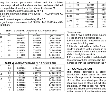
Observations
1. Table 1 revels that the total expense is positive sensitive w. r. t. the change in ordering cost.
2. From table 2 it is noticed that the total cost is rises with the increment in holding cost.
3. It is also noticed from tables 3 and 4 that the total cost is positive sensitive to the change in demand parameters. It is observed that the demand parameter a is highly sensitive while b is slightly sensitive.
4. From table 5 and 6, it is detected that the expense is decreasing with the increment in the interest earned while it is increases with the increment in the rate of interest charged.
IV.
CONCLUSION
This article addresses a problem, for time varying deteriorating items under the circumstance in which the demand is supposed to be exponentially increasing function of time. We have developed the paper with some realistic situations such as stock out, which is unavoidable in certain situations. In this model we have investigated the article under the inflationary conditions under the reasonable delay in the payment. A mathematical model has been created to find the best possible replenishment policies. The problem is analyzed with some numerical investigations to justify our model and the influences of the deviation of some input parameters has been studied in the sensitivity analysis.
REFERENCES
[1] Aggarwal S.P., Jaggi C.K. (1995). Ordering policies of deteriorating items under permissible delay in payments, Journal of Operational Research of Society, vol.46, pp.658-662.
[2] Benkherouf L., (1995). On an inventory model with deteriorating items and decreasing time-varying demand and shortages, European Journal of Operational Research, vol.86, pp.293-299.
[3] Dem, H., Singh, S., & Kumar, J. (2014). An EPQ model with trapezoidal demand under volume flexibility. International Journal of Industrial Engineering Computations, 5(1), 127-138.
[4] Ghare P.M., Schrader G.H., (1963). A model for exponentially decaying inventory system, International Journal of Production Research, vol.21, pp.449-460. [5] Goyal, S.K., (1985) Economic order quantity under
conditions of permissible delay in payments, Journal of Operational Research Society, vol.36, pp.335-338. [6] 6. Goyal, S.K., Giri, B.C. (2001). Recent trends in
modeling of deteriorating inventory, European, Journal of Operational Research, vol.134, pp.1-16.
[7] Kumar J., Singh S.R., (2012). An Inventory model with volume flexible process under inflation and shortages. International transactions in mathematical sciences and computers, 5(2), (333-340).
horizon. Journal of Advanced Research in Dynamical and Control Systems 11(6 Special Issue), 108-119. [9] Kumar, S., Handa, N., Singh, S. R., & Yadav, D. (2015).
Production inventory model for two-level trade credit financing under the effect of preservation technology and learning in supply chain. Cogent Engineering, 2(1), 1045221.
[10]Saxena, N., Singh, S. R., & Sana, S. S. (2017). A green supply chain model of vendor and buyer for remanufacturing. RAIRO-Operations Research, 51(4), 1133-1150.
[11]Singh S.R., Kumar J., (2010). Two warehouse inventory model for deteriorating items with stock dependent demand and shortages under the condition of permissible delay. International journal of mathematical sciences, 9(3-4), (415-431).
[12]Singh S.R., Singh, N. (2009). A Production Inventory Model with Variable Demand Rate for Deteriorating Items under Permissible Delay in Payments, International Transactions in Mathematical Sciences and Computer, vol.2 and vol.1, pp. 73-82.
[13]Singh S.R., Singh, S. (2010). An Optimal Inventory Policy For Items Having Linear Demand And Variable Deterioration Rate With Trade Credit, International Journal of Management Research and Technology, vol.4, pp. 293-298.
[14]Yadav, A.S., Bansal, K.K., Kumar, J., Kumar, S. (2019). Supply chain inventory model for deteriorating item with warehouse & distribution centers under inflation. International Journal of Engineering and Advanced Technology. 8(2), pp. 7-13
[15]Yadav, A.S., Kumar, J., Malik, M., Pandey, T. (2019). Supply chain of chemical industry for warehouse with distribution centers using artificial bee colony algorithm. International Journal of Engineering and Advanced Technology. 8(2), 14-19.