https://doi.org/10.5194/nhess-17-1763-2017 © Author(s) 2017. This work is distributed under the Creative Commons Attribution 3.0 License.
Variations in return value estimate of ocean surface waves – a study
based on measured buoy data and ERA-Interim reanalysis data
T. Muhammed Naseef and V. Sanil Kumar
Ocean Engineering Division, Council of Scientific and Industrial Research (CSIR)–National Institute of Oceanography, Dona Paula 403 004, India
Correspondence to:V. Sanil Kumar ([email protected]) Received: 9 May 2017 – Discussion started: 19 June 2017 Accepted: 12 September 2017 – Published: 19 October 2017
Abstract. An assessment of extreme wave characteristics during the design of marine facilities not only helps to en-sure their safety but also assess the economic aspects. In this study, return levels of significant wave height (Hs) for dif-ferent periods are estimated using the generalized extreme value distribution (GEV) and generalized Pareto distribution (GPD) based on the Waverider buoy data spanning 8 years and the ERA-Interim reanalysis data spanning 38 years. The analysis is carried out for wind-sea, swell and totalHs sepa-rately for buoy data. Seasonality of the prevailing wave cli-mate is also considered in the analysis to provide return lev-els for short-term activities in the location. The study shows that the initial distribution method (IDM) underestimates re-turn levels compared to GPD. The maximum rere-turn lev-els estimated by the GPD corresponding to 100 years are 5.10 m for the monsoon season (JJAS), 2.66 m for the pre-monsoon season (FMAM) and 4.28 m for the post-pre-monsoon season (ONDJ). The intercomparison of return levels by block maxima (annual, seasonal and monthly maxima) and the r-largest method for GEV theory shows that the maxi-mum return level for 100 years is 7.20 m in ther-largest se-ries followed by monthly maxima (6.02 m) and annual max-ima (AM) (5.66 m) series. The analysis is also carried out to understand the sensitivity of the number of observations for the GEV annual maxima estimates. It indicates that the variations in the standard deviation of the series caused by changes in the number of observations are positively cor-related with the return level estimates. The 100-year return level results ofHsusing the GEV method are comparable for short-term (2008 to 2016) buoy data (4.18 m) and long-term (1979 to 2016) ERA-Interim shallow data (4.39 m). The 6 h interval data tend to miss high values ofHs, and hence there
is a significant difference in the 100-year return levelHs ob-tained using 6 h interval data compared to data at 0.5 h inter-val. The study shows that a single storm can cause a large difference in the 100-yearHsvalue.
1 Introduction
which incorporates the peak over threshold (POT) approach (Pickands, 1975; Coles et al., 2001).
GEV distribution by annual maxima (AM) observations (Goda, 1992) is one of the widely used methods in the EVT analysis. The main difficulty with using this method is the unavailability of reliable observations at a location of inter-est. To overcome the data scarcity, two different alternatives have been used by various authors: (i) the initial distribu-tion method (IDM), in which all the data are used (Alves and Young, 2003); and (ii) ther-largest approach (Smith, 1986), where a number of the largest observations from a block pe-riod are considered rather than one observation as used in the AM method. The POT method (Abild et al., 1992) provides a good number of observations available for the analysis. Al-though there have been various proposals to automate thresh-old selection, threshthresh-old estimation for the application of the POT method to a single sample is still not resolved (Solari and Losada, 2012; Solari et al., 2017). GPD is another class of distribution introduced by Pickands (1975) and has been used by several authors such as Caires and Sterl (2005) and Thevasiyani et al. (2014). Teena et al. (2012) and Samayam et al. (2017) have carried out the EVT analysis of ocean sur-face waves in the northern Indian Ocean based on wave hind-cast data and ERA-Interim reanalysis data.
The most reliable source of ocean wave data is buoy mea-surements, and it can be used for EVT analysis (Panchang et al., 1999). In this paper, data from a directional Waverider buoy located in the central western shelf of India are used. Seasonality is one of the important aspects of climate data, and, therefore, it should be incorporated in the EVT anal-ysis of waves, especially in a region such as the Arabian Sea. Seasonal analysis of the extremes helps in the planning of short-term marine activities such as offshore explorations and maintenance of coastal facilities. In the present paper, the EVT analysis is carried out by following both the GEV and GPD methods considering wind-sea, swell and total signifi-cant wave height (Hs) separately. The IDM and POT methods are used for total wave height analysis, and block maxima (annual and monthly maxima) and ther-largest method are used in wind-sea and swell height analysis. Since the mea-sured buoy data are for a short period of 8 years, the ERA-Interim reanalysis data from 1979 to 2016 are also used for comparing theHsvalue with the 100-year return period.
The paper is organized as follows. Section 2 deals with the data and methodology used in the analysis. It also presents the threshold selection adopted in the study, and Sect. 3 ex-plains the results obtained in the analysis, categorized into seasons using total Hs data, and comparison of return level estimation by different GEV approaches using wind-sea and swell height data. A case study is also included in the sec-tion for realizing the uncertainty related to observasec-tions in the AM approach when a limited number of observations are available. The influence of length of wave data on the es-timated Hs return value is also covered under this section. Section 4 provides the concluding remarks.
2 Data and methodology 2.1 Data
Data used in the analysis are from a Datawell directional Wa-verider buoy deployed off Honnavar (14.304◦N; 74.391◦E) at a water depth of 9 m. The half-hourly sampled data cover the period from March 2008 to February 2016. The waves at the location show strong intra-annual variations due to the prevailing wind system during monsoon and non-monsoon seasons (Sanil Kumar et al., 2014). To understand the local and remote influences on the design wave characteristics, we analyzedHs of wind-sea, swell and total waves separately. A season-wise study is also carried out since it will provide insight into the design wave heights for short-term coastal activities.
The Hs data from ERA-Interim (Dee et al., 2011), the global atmospheric reanalysis product of the European Cen-tre for Medium-Range Weather Forecast (ECMWF), from 1979 to 2016 (38 years) are also used to evaluate the 100-and 50-year return period wave height in the shallow (water depth∼20 m) and deep water. The shallow region is close to the buoy location, and the deep water location is at a wa-ter depth of∼4000 m (Table 1). The ERA-Interim reanalysis used in the study has a spatial resolution of 0.125◦×0.125◦ and a temporal resolution of 6 h.
2.2 Methodology
EVT analysis is carried out by following the GEV distribu-tion model and the POT method in which exceedance over a reliable threshold wave height can be fit into GPD. In the POT method, distribution of excess,x, over a thresholduis defined as
Fu(y)=Pr{x−u ≤x|x > u} =
F (x)−F (u)
1−F (u) , (1)
wherey=x−u. Pickands (1975) shows that the distribution function of excess,Fu(y), for a sufficiently high thresholdu converges to GPD, having a cumulative distribution function (CDF) as follows:
G (x;k, α, β)= {1−
1−kx−β α
1/k
} k6=0 (2)
=1−e−(x−β)/α k=0. (3) GEV has a CDF as follows:
F (X)=exp (
−(1−k
X−β α
1/k)
k6=0 (4)
=exp
−exp(−X−β
α )
k=0, (5)
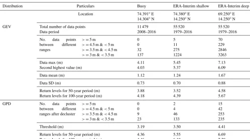
Table 1.The comparison of 50- and 100-year significant wave height return levels based on buoy, ERA-Interim shallow and ERA-Interim deep data at 6 h intervals along with data statistical parameters.
Distribution Particulars Buoy ERA-Interim shallow ERA-Interim deep
Location 74.391◦E
14.304◦N
74.380◦E 14.250◦N
69.250◦E 14.250◦N
GEV Total number of data points Data period 11 479 2008–2016 55 520 1979–2016 55 520 1979–2016
No. data points between different ranges
>=5 m
>=4.5 m &<5 m >=3.5 m &<4.5 m >=3 m &<3.5 m
0 0 32 137 5 11 275 1224 70 229 2846 3263
Data max (m)
Second highest value (m)
4.11 4.03 5.45 5.37 7.13 6.09
Data mean (m) 1.12 1.24 1.67
Data SD (m) 0.73 0.70 0.88
Return levels for 50-year period (m) Return levels for 100-year period (m)
3.88 4.18 3.52 4.39 4.58 5.67
GPD No. data points
between different ranges after decluster
>=5 m
>=4.5 m &<5 m >=3.5 m &<4.5 m >=3 m &<3.5 m
0 0 9 23 2 4 46 133 15 42 253 235
Threshold (m) 3.19 3.50 4.41
Return levels for 50-year period (m) Return levels for 100-year period (m)
4.36 4.46 5.55 6.18 6.69 7.28
kis the shape parameter in the range of−∞< k <∞. GPD can be further categorized into three distributions based on its tail features. Whenk=0, GPD corresponds to an exponen-tial distribution (medium-tailed or Pareto type I) with mean α; when k >0, GPD is short-tailed, also known as Pareto type II; when k <0, the distribution takes the form of or-dinary Pareto distribution, having a long-tailed distribution (also known as Pareto type III). Parameter estimation and sta-tistical distribution fitting are carried out by using the WAFO toolbox (Brodtkorb et al., 2000), developed by Lund Univer-sity, Sweden.
The analysis is carried out by using the wind-sea, swell and total Hs data covering ∼8 years (2008–2016). From the measured data, to separate the wind seas and swells, the method proposed by Portilla et al. (2009) is used. The sepa-ration algorithm is based on the assumption that the energy at the peak frequency of a swell cannot be higher than the value of a Pierson–Moskowitz (PM) spectrum with the same frequency. If the ratio between the peak energy of a wave system and the energy of a PM spectrum at the same fre-quency is above a threshold value of 1, the system is con-sidered to represent wind sea – otherwise it is taken to be a swell. A separation frequency fc is estimated following Portilla et al. (2009), and the swell and wind-sea parame-ters are obtained for frequencies ranging from 0.025 Hz to fc and fromfcto 0.58 Hz respectively. The GPD method is used for seasonal analysis of different period data series. The
GEV method is used for intercomparison of return level esti-mation among wind-sea, swell and resultant data sets by ex-tracting different block maxima series: (i) seasonal maxima, which contain the highest observations from each season; (ii) monthly maxima, which contain one highest observa-tion from each month; and (iii) annual maxima. The param-eters are estimated using the probability-weighted moment (PWM) method since the data set duration is very limited, and the PWM method holds good results compared to other methods such as the maximum likelihood method (Hosking et al., 1985).
To study the uncertainties related to the length of the ob-servation, we extracted 3, 6, 12 and 24 h data series from the half-hourly original data and carried out EVT analysis. Since the wave climate in the study location is strongly char-acterized by the prevailing seasonal behavior of wind sys-tem, we took further consideration of uncertainties related to a seasonal aspect of wave climate by extracting three sea-sonal data sets, viz. pre-monsoon (FMAM), monsoon (JJAS) and post-monsoon (ONDJ) seasons.
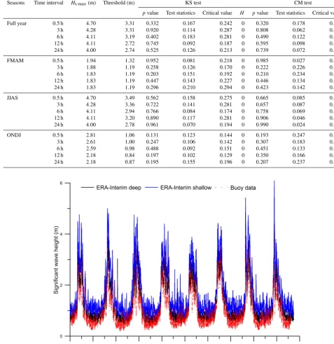
Table 2.Different goodness of fit tests used for selecting threshold values of POT analysis.H=0 indicates that the test does not reject the hypothesis at the 5 % significance level (i.e.,p value>0.05 or test statistics is less than critical value), andH=1 indicates that the hypothesis is rejected. KS test represents the Kolmogorov–Smirnov test and CM test represents the Cramér–von Mises test.
Seasons Time interval Hs-max(m) Threshold (m) KS test CM test
pvalue Test statistics Critical value H pvalue Test statistics Critical value H
Full year 0.5 h 4.70 3.31 0.332 0.167 0.242 0 0.320 0.178 0.459 0 3 h 4.28 3.31 0.920 0.114 0.287 0 0.808 0.062 0.458 0 6 h 4.11 3.19 0.402 0.183 0.281 0 0.490 0.122 0.458 0 12 h 4.11 2.72 0.745 0.092 0.187 0 0.595 0.098 0.460 0 24 h 4.00 2.74 0.525 0.126 0.213 0 0.739 0.072 0.459 0 FMAM 0.5 h 1.94 1.32 0.952 0.081 0.218 0 0.985 0.027 0.459 0 3 h 1.88 1.19 0.258 0.126 0.170 0 0.222 0.226 0.460 0 6 h 1.83 1.19 0.203 0.151 0.192 0 0.210 0.234 0.460 0 12 h 1.83 1.19 0.447 0.143 0.227 0 0.446 0.134 0.459 0 24 h 1.83 1.19 0.296 0.210 0.294 0 0.423 0.142 0.458 0
JJAS 0.5 h 4.70 3.49 0.562 0.158 0.275 0 0.665 0.085 0.458 0 3 h 4.28 3.36 0.722 0.141 0.281 0 0.657 0.087 0.458 0 6 h 4.11 2.94 0.766 0.084 0.174 0 0.758 0.069 0.460 0 12 h 4.11 3.20 0.890 0.117 0.281 0 0.906 0.046 0.458 0 24 h 4.00 2.78 0.961 0.070 0.194 0 0.990 0.024 0.460 0
ONDJ 0.5 h 2.81 1.06 0.131 0.123 0.144 0 0.193 0.247 0.460 0 3 h 2.61 1.00 0.247 0.106 0.142 0 0.307 0.183 0.460 0 6 h 2.59 0.98 0.488 0.092 0.151 0 0.451 0.133 0.460 0 12 h 2.18 0.84 0.197 0.102 0.129 0 0.350 0.166 0.461 0 24 h 2.18 0.87 0.195 0.155 0.196 0 0.207 0.237 0.460 0
Figure 1.Time series plot of the significant wave height measured by buoy and from ERA-Interim data at shallow and deep water.
EVT is based on the assumption that the observations un-der consiun-deration are independent and identically distributed (Coles et al., 2001). We can expect identical status of ocean wave observations for a large extent. Since the POT approach resamples the data over a threshold value, making identical and independent observations is a tedious task. A suitable
combination of threshold and minimum separation time be-tween the resampled observations must be taken into account to establish independence among the observations.
Figure 2.Estimated shape parameters for different seasonal data with different sampling intervals used in the(a)GEV and(b)GPD model.
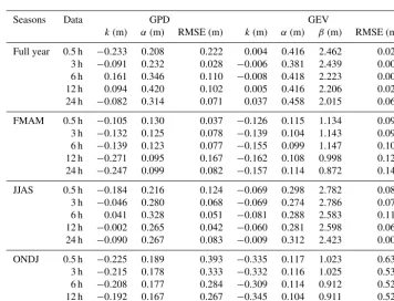
Table 3.Table showing different parameters and corresponding RMSEs of data and the estimated CDF used during each data series analysis.
Seasons Data GPD GEV
k(m) α(m) RMSE (m) k(m) α(m) β(m) RMSE (m)
Full year 0.5 h −0.233 0.208 0.222 0.004 0.416 2.462 0.023 3 h −0.091 0.232 0.028 −0.006 0.381 2.439 0.008 6 h 0.161 0.346 0.110 −0.008 0.418 2.223 0.004 12 h 0.094 0.420 0.102 0.005 0.416 2.206 0.020 24 h −0.082 0.314 0.071 0.037 0.458 2.015 0.060
FMAM 0.5 h −0.105 0.130 0.037 −0.126 0.115 1.134 0.090 3 h −0.132 0.125 0.078 −0.139 0.104 1.143 0.098 6 h −0.139 0.123 0.077 −0.155 0.099 1.147 0.100 12 h −0.271 0.095 0.167 −0.162 0.108 0.998 0.125 24 h −0.247 0.099 0.082 −0.157 0.114 0.872 0.142
JJAS 0.5 h −0.184 0.216 0.124 −0.069 0.298 2.782 0.088 3 h −0.046 0.280 0.068 −0.069 0.274 2.786 0.074 6 h 0.041 0.328 0.051 −0.081 0.288 2.583 0.118 12 h −0.002 0.265 0.042 −0.060 0.281 2.598 0.065 24 h −0.090 0.267 0.083 −0.009 0.312 2.423 0.007
ONDJ 0.5 h −0.225 0.189 0.393 −0.335 0.117 1.023 0.631 3 h −0.215 0.178 0.333 −0.332 0.116 1.025 0.533 6 h −0.208 0.177 0.284 −0.309 0.114 0.912 0.525 12 h −0.192 0.167 0.267 −0.345 0.104 0.911 0.523 24 h −0.251 0.183 0.315 −0.334 0.111 0.780 0.498
between two consecutive storm peaks to ensure the indepen-dence of the data points for the analysis. Then, we selected a tentative threshold value in such a way as to ensure the presence of at least 15 peak values per year on average. This resulted in at least 120 data points in each sub-data sets used for the seasonal analysis. The resulting data series are used in further POT analysis. Further adjustment of the threshold
Figure 3.Typical(a)SME and(b)PS plots used for selecting a range of thresholds required for POT analysis. In this particular case, a range of 1.19 to 1.32 m was selected.
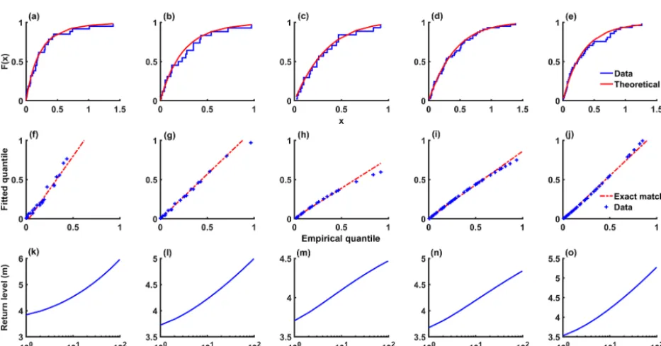
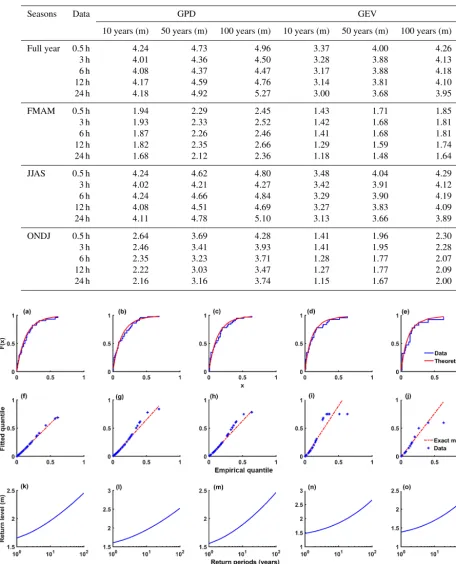
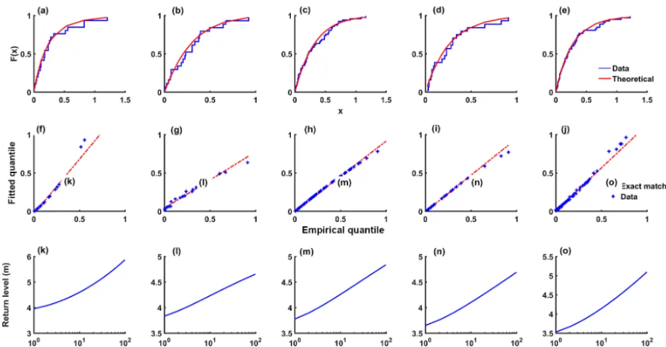
Figure 4.Figure corresponding to the full-year analysis.(a)to(e)represent the CDF plots for half, 3, 6, 12 and 24-hourly data respectively; (f)to(j)correspond toQ-Qplots;(k)to(o)correspond to return levels estimated using the GPD model.
(AD) test and Cramér–von Mises (CM) test (Stephens, 1974; Choulakian and Stephens, 2001).
The distributions used in the analysis are validated using graphical tools such as quantile–quantile (Q-Q) plots and CDF plots. In addition to above graphical tools, we checked the reliability of the chosen thresholds for the POT method by using different GOF tests such as KS, AD and CM tests (Table 2). Apvalue>0.05 indicates that the selected distri-bution does not show a significant difference from the origi-nal data within the 5 % significance interval.
3 Results and discussion
3.1 Long-term statistical analysis of totalHs
Table 4.Estimated return values corresponding to different seasons using total wave height (Hs) following the GEV and GPD methods. Here the GEV method follows the initial distribution approach.
Seasons Data GPD GEV
10 years (m) 50 years (m) 100 years (m) 10 years (m) 50 years (m) 100 years (m)
Full year 0.5 h 4.24 4.73 4.96 3.37 4.00 4.26
3 h 4.01 4.36 4.50 3.28 3.88 4.13
6 h 4.08 4.37 4.47 3.17 3.88 4.18
12 h 4.17 4.59 4.76 3.14 3.81 4.10
24 h 4.18 4.92 5.27 3.00 3.68 3.95
FMAM 0.5 h 1.94 2.29 2.45 1.43 1.71 1.85
3 h 1.93 2.33 2.52 1.42 1.68 1.81
6 h 1.87 2.26 2.46 1.41 1.68 1.81
12 h 1.82 2.35 2.66 1.29 1.59 1.74
24 h 1.68 2.12 2.36 1.18 1.48 1.64
JJAS 0.5 h 4.24 4.62 4.80 3.48 4.04 4.29
3 h 4.02 4.21 4.27 3.42 3.91 4.12
6 h 4.24 4.66 4.84 3.29 3.90 4.19
12 h 4.08 4.51 4.69 3.27 3.83 4.09
24 h 4.11 4.78 5.10 3.13 3.66 3.89
ONDJ 0.5 h 2.64 3.69 4.28 1.41 1.96 2.30
3 h 2.46 3.41 3.93 1.41 1.95 2.28
6 h 2.35 3.23 3.71 1.28 1.77 2.07
12 h 2.22 3.03 3.47 1.27 1.77 2.09
24 h 2.16 3.16 3.74 1.15 1.67 2.00
Figure 5.Same as in Fig. 4 but corresponding to the pre-monsoon season.
that of Anoop et al. (2015) reported that averageHs attains its peak at around 3 m during JJAS and that the FMAM sea-son is relatively calm (0.5–1.5 m) compared to ONDJ (1.5–
Figure 6.Same as in Fig. 4 but corresponding to the monsoon season.
than block maxima (Mathiesen et al., 1994). One of the chal-lenging tasks for GPD modeling is the selection of a suit-able threshold value. The threshold should be high enough for observations to be independent, and data after POT anal-ysis must have the necessary number of observations in order to converge the POT analysis into GPD. SME plots and PS plots are used to select a range of initial thresholds. Upon analyzing the resultant GPD fit for those thresholds, the fi-nal thresholds are chosen with the help of GOF tests, which are presented in Table 2. Figure 2 and Table 3 show the es-timated parameters using the PWM method for both GEV and GPD. It is clear that shape parameters in both cases are negative, indicating that the models are a type III distribution for GPD and a Weibull distribution for GEV. Table 3 also shows the RMSE in the chosen model for each data series with estimated CDF. It is evident that the JJAS season has a lower RMSE (∼0.07 m on average) when considering the GPD model, while, in the case of the GEV model, the full-year data series has a lower RMSE (∼0.02 m on average). The ONDJ season shows a higher discrepancy in both cases, resulting in an average RMSE of 0.31 and 0.54 m for GPD and GEV respectively. Figure 3 shows the typical SME and PS plots used for choosing a range of thresholds before fix-ing the final threshold for POT analysis on each series. In this particular case (6 h data series of FMAM season), a range of thresholds from 1.10 to 1.32 m was selected, and the final threshold of 1.19 m was fixed for analyzing the GOF test re-sults (Table 2).
3.1.1 Full year
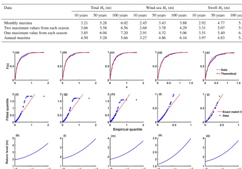
respec-Table 5.Return levels estimated by the GEV model using total, wind-sea and swell data for different block maxima series.
Data TotalHs(m) Wind-seaHs(m) SwellHs(m)
10 years 50 years 100 years 10 years 50 years 100 years 10 years 50 years 100 years
Monthly maxima 3.21 5.28 6.02 2.45 3.43 3.88 2.92 4.77 5.72 Two maximum values from each season 3.66 5.58 6.56 2.68 3.78 4.29 3.31 5.07 5.95 One maximum value from each season 3.85 6.04 7.20 2.91 4.32 5.06 3.51 5.40 6.35
Annual maxima 4.50 5.28 5.66 3.27 4.86 6.16 3.97 4.83 5.35
Figure 7.Same as in Fig. 4 but corresponding to the post-monsoon season.
tively. When considering different time interval data, both 12 and 24 h data series estimate lower return levels compared to other series by the GEV model. It is evident that there are uncertainties related to the sampling interval adopted for the return value estimation. The standard deviation for GPD es-timation when considering different time intervals is 0.57 m, which is highest among the other seasonal data. GEV estima-tion reports an even lower spread of return levels with 0.16 m standard deviation.
3.1.2 Pre-monsoon season
The data from February to May constitute the pre-monsoon data set. Pre-monsoon is the calmest season in the study lo-cation, with a maximum and an averageHs of around 1.94 and 0.73 m respectively. Using SME and PS plots, a range of thresholds from 1.19 to 1.32 m is selected for each time series and fitted to the corresponding GPD by using the re-sultant POT values. The final threshold selected by the help of GOF tests is presented in Table 2. KS and CM tests give a p value of more than 0.43 and 0.45 respectively on average (Table 2). Since thepvalues are more than 0.05, the chosen
POT is not significantly different from the time series data. CDF plots andQ-Qplots (Fig. 5) for the different data series of the season illustrate the reliability of the chosen model. Return levels for different return periods using a particular GPD are presented in Table 4. GEV estimation exhibits the same characteristics of underestimation as shown in the full-year analysis. Average 100-full-year return levels estimation us-ing different time interval data usus-ing the GEV model attained a value of only 1.77 m, which is less than the highest ob-served data point in the season, whereas GPD reports an av-erage 100-year return level of 2.49 m. Time interval analysis for the season exhibits the least discrepancies among the re-turn level estimations compared to other seasons. Standard deviations of 0.11 and 0.08 m for GPD and GEV estimations respectively were observed for 100-year return levels consid-ering different time series data.
3.1.3 Monsoon season
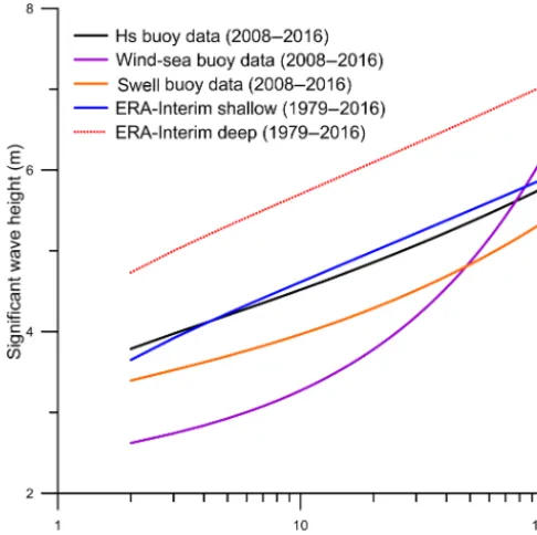
Figure 8.Return levels of significant wave heights for different re-turn periods based on buoy data (2008–2016), ERA-Interim shallow water data and ERA-Interim deep water data (1979–2016) at 6 h in-tervals by the GEV model using annual maxima series.
are recorded for the maximum and average respectively dur-ing the season. A range of thresholds (2.78 to 3.49 m) is se-lected for preliminary GPD fitting as a result of interpreting SME and PS plots of each data series, and the correspond-ing final thresholds were selected after clarifycorrespond-ing with the GOF test results (Table 2). Both KS and CM tests report a p value>0.56, indicating that the resulting POT series for the selected threshold converges into GPD. CDF and Q-Q plots in Fig. 6 shows the reliability of the adopted threshold value. Return levels for the distinct return period were esti-mated using the resultant POT series. Table 4 provides 10-, 50- and 100-year return period values estimated using GPD and GEV models. For half-hourly data, GPD projects a value of 4.80 m for the 100-year return level, whereas GEV under-estimates it, with a value of 4.29 m. The GPD model shows a 0.36 m standard deviation among the return levels for differ-ent time interval data. Both the 12 and 24 h series gave lower return levels compared to other series.
3.1.4 Post-monsoon season
The post-monsoon season constitutes data from the October to January months of the year, and the observed maximum Hs in this season is 2.41 m. The majority of observations during this season lie below the average value ofHs. Only 32 % of the observations lie above 1.13 m, and 8 % of the data are above 1.5 m. Hence, selecting the best threshold for the season was more difficult. GPD was fitted for a range of
thresholds (0.7 to 1.3 m) selected from SME and PS plots corresponding to each series. Most suitable thresholds were selected after checking the goodness of fit of GPD (Table 2). The GOF test results show that the ONDJ series holds maxi-mum uncertainties on threshold selection due to lowerp val-ues for the KS test ranges from 0.13 to 0.48 and from 0.19 to 0.45 for the CM test. Figure 7 shows the CDF andQ-Q plots. The GEV and GPD estimations for the post-monsoon season show very large difference among return levels (Ta-ble 4). The average percentage difference between the 100-year return values obtained from GEV and GPD estimations is∼60 %. This shows that the GEV model clearly under-performs during the ONDJ season, when the initial distribu-tion methods were adopted. The highest return level reported by the GPD model is 4.28 m, whereas GEV estimated about 2.3 m for the season. The ONDJ season has a standard devi-ation of 0.30 and 0.13 m for the GPD and GEV estimdevi-ation respectively while using different sampling intervals. 3.2 Long-term statistical analysis of wind seas and
swells
Figure 9.Density plots showing the probability for different wave height class. Total, wind-sea and swellHsare presented row wise. Columns correspond to the selected number of data points (5 to 8 years). The solid curve is the corresponding GPD fit.
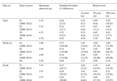
Table 6.Table showing the results of the case study. The standard deviations (SDs) of each data series considered are provided, and percentage differences among the SDs of each series with parent series (S0) are given in the brackets. The percentage difference in the corresponding return level estimation is also shown in the brackets of the respective return periods.
Data set Series (years) Maximum observed (m) Standard deviation (% difference) Return levels 10 years (m) 50 years (m) 100 years (m) Total S1 (2008–2012) 4.32 0.36 (21.8) 4.24 (6.1) 4.89 (8.6) 5.20 (10.42) S2 (2008–2013) 4.32 0.32 (32.7) 4.17 (8.0) 4.67 (13.1) 4.90 (15.5) S3 (2008–2014) 4.32 0.32 (34.5) 4.23 (6.4) 4.65 (13.5) 4.83 (17.2)
S0 4.70 0.45 4.50 5.28 5.66
Wind sea S1
(2008–2012) 2.80 0.13 (128.90) 2.82 (14.81) 2.88 (51.29) 2.89 (72.30) S2 (2008–2013) 2.80 0.14 (125.06) 2.81 (15.00) 2.95 (48.96) 3.00 (69.16) S3 (2008–2014) 2.89 0.16 (114.08) 2.89 (12.35) 3.05 (45.80) 3.11 (66.00)
S0 4.29 0.60 3.27 4.86 6.16
Swell S1 (2008–2012) 3.47 0.23 (48.17) 3.65 (8.23) 4.16 (14.93) 4.45 (18.36) S2 (2008–2013) 3.47 0.20 (58.53) 3.62 (9.18) 4.01 (18.53) 4.22 (23.56) S3 (2008–2014) 3.47 0.22 (50.80) 3.71 (6.62) 4.05 (17.53) 4.21 (23.97)
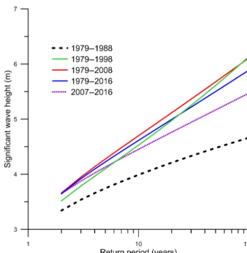
Figure 10.Return levels of significant wave heights for different return periods based on ERA-Interim shallow water data in different block years by the GEV model using annual maxima series.
correlated with standard deviation (Table 6). In the case of the total Hs, the correlation between the changes in stan-dard deviation and the corresponding changes in 100-year re-turn levels is 0.997, whereas for wind sea and swell they are 0.964 and 0.647 respectively. The annual maxima of wind sea (4.29 m) for the year 2015 caused an abrupt change in the standard deviation of the series by about 0.46 m, which is more than 17 % of the average of the series excluding 2015. Therefore, the 100-year return level for wind sea overshoots by about 6.16 m, resulting in a 66 % difference from return value obtained for S3 series. In this case study, the length of the special series under consideration does not influence the estimated return levels; that is, in the case of the totalHs se-ries, the 100-year return level for the S1 series is greater than for both the S2 and S3 series. The same characteristics can also be seen in the case of swellHs. Therefore, return levels for annual maxima by the GEV model have greater influence over how a single data point, i.e., the annual maxima, alters the standard deviation of the series rather than the changes in the length of the series.
3.3 Influence of length of wave data on the estimated significant wave height return value
An analysis is carried out to check uncertainties in return level estimation related to the length of the wave record. From the 0.5 h buoy-measured data, data at 6 h intervals are extracted and used for the analysis, and the return lev-els obtained by using 6 h measured buoy data are compared
with the return level obtained from the 6 h ERA-Interim data at shallow and deep locations (Fig. 8). The 6-hourly ERA-Interim reanalysis 38-year data (1979–2016) are used in this analysis. Buoy data consist of 11 479 data points, and ERA-Interim data consist of 55 520 data points (Table 1). The high-est observedHsin the 6-hourly buoy data is 4.11 m followed by 4.03 m, while the maximumHs in ERA-Interim shallow water is 5.45 m and in ERA-Interim deep water it is 7.13 m. TheHsvalues at the deep location are∼1.4 times the values at the shallow location, and this resulted in a higher return level ofHsat the deep location. Sanil Kumar and Muhammed Naseef (2015) observed that ERA-Interim overestimates the Hs for shallow water locations along the west coast of In-dia due to swell height overestimation, and the difference be-tween the ERA-InterimHsand the buoyHsis up to 15 %. For the study location, the storm-induced wave heights during the non-monsoon period are less than the monsoon-induced waves. The 1st week of June is the onset of the Indian sum-mer monsoon, and the maximum Hs in the study area is due to monsoon influence; in all years, this occurs during June to September. The 100-year return levels using the GEV method are comparable for buoy data (4.18 m) and ERA-Interim shallow data (4.39 m), while that for ERA-ERA-Interim deep is 5.67 m (Fig. 8). It is clear that the 100-yearHs re-turn level using GEV for ERA-Interim data is lower than the maximumHsin the data, while, in the case of buoy data, the 100-year return level is slightly higher than the highestHs value. The return levels obtained by the GPD method show significant discrepancy among year estimates. The 100-year return level obtained for buoy data is 4.46 m, but that using Interim shallow data is 6.18 m and that for ERA-Interim deep is 7.28 m. The 100-yearHsreturn level for deep water has closer values following GEV and GPD, while, in the shallow water, a significant difference is obtained. The 6 h interval data tend to miss 18 values ofHsbetween 4.11 and 4.70 m, and hence there is a significant difference in the 100-year return level ofHsbased on GEV-AM obtained us-ing these data compared to that based on the data at 0.5 h intervals.
Figure 11. Variation of the(a)annual maximum and(b) annual meanHsat the shallow locations based on ERA-Interim data. The solid line indicates the trend inHsduring 1979 to 2016.
the 100-year Hs value compared to the 38-year data. If we consider only the last 10 years (2007–2016), it resulted in a 7 % underestimation in the 100-year Hs value. The study shows that a single storm can create a large difference in the 100-yearHsvalue, compared to the differences in values that resulted from a different length of the data block.
The long-term and decadal trend of wave climate in the different parts of major oceans is studied (Young et al., 2011). We have examined the trend in Hs at the shallow location based on the ERA-Interim data from 1979 to 2016. The study shows that the annual maximumHsshows a weak in-creasing trend (1.1 cm yr−1), whereas there is no significant trend in the annual mean value (Fig. 11). Sanil Kumar and Anoop (2015) observed that during 1979 to 2012 the average trend of annual meanHs for all the locations in the western shelf seas was 0.06 cm yr−1.
3.4 Influence of water depth on the measured buoy data
The relative water depth based on the spectral peak period (d/Lp)indicates that most of the time (97.8 to 99.3 %) the wave regime is in intermediate water (Table 7). Only dur-ing 0.1 to 0.8 % of the time do the waves satisfy the deep water condition. Hence, the waves measured by the buoys are influenced by the bathymetry, and the wave characteris-tics are different in the deep water. The wave rose plots from March 2008 to February 2016 based on the measured buoy data and the ERA-Interim reanalysis data at shallow and deep water locations are presented in Fig. 12. As the waves move from deep to shallow waters, the direction of high waves shifted from southwest to west. The limiting value of wave height based on breaker criteria is 0.6 to 0.78 times the wa-ter depth (Massel, 1966). The maximumHsin the measured
Figure 12.Wave rose plots from March 2008 to February 2016 based on the measured buoy data and the ERA-Interim reanalysis data at shallow and deep water locations.
buoy data is 4.70 m, and some of the waves containing this record are very steep or broken at 9 m water depth since the maximum wave height is 1.65 to 1.8 times theHs.
4 Conclusions
appro-Table 7.The percentage of time of the waves in the shallow, intermediate and deep water regime in different years along with the mean wave period and mean peak wave period.
Year Mean wave period (s) Criteria based on ratio of water depth and wave length
corresponding to mean wave period
Mean peak wave period (s) Criteria based on ratio of water depth and wave length
corresponding to peak wave period
Shallow Intermediate Deep Shallow Intermediate Deep
water water water water water water
2008–2009 5.5 0 98.7 1.3 12.1 1.0 98.9 0.1
2009–2010 5.6 0 98.3 1.6 12.0 0.5 99.3 0.2
2010–2011 5.4 0 97.5 2.5 11.7 0.6 99.2 0.2
2011–2012 5.7 0 99.5 0.5 11.9 0.9 98.5 0.6
2012–2013 5.5 0 99.4 0.6 12.0 0.3 99.6 0.1
2013–2014 5.0 0 95.0 5.0 11.8 1.4 97.8 0.8
2014–2015 5.7 0 98.7 1.3 12.6 1.8 98.1 0.1
2015–2016 5.5 0 98.0 2.0 12.3 0.8 99.0 0.2
priate thresholds for the POT method is justified using dif-ferent GOF tests results. Analysis of the totalHsshows that the IDM approach underestimates return levels for different seasons compared to the corresponding GPD. The 100-year return levels estimated by IDM are almost comparable with the corresponding GPD estimation for the 10-year period, but there is a significant difference in the return level esti-mates when considering different sampling intervals. IDM estimates largely underestimate return levels for the post-monsoon season since the majority of the observation in this season lies away from its tail of the distribution.
Long-term statistics of wind-sea and swell data are cal-culated by the GEV model following block maxima and ther-largest methods. Annual maxima and monthly maxima are considered for block maxima series, and two seasonal maxima series are considered for ther-largest method. It is shown that these methods give higher return levels than the GPD models. The the r-largest method provides 7.20 m as the 100-year return level when compared to 5.27 m of the GPD model. The sensitivity analysis of the GEV-AM model shows that change in the standard deviation of data series under consideration causes discrepancies in the return level estimates rather than a change in the length of the series. Both GEV and GPD models underestimate 10-year return levels compared to maximum measured data. The 100-year return levels acquired by using the GEV method are com-parable for short-term (2008 to 2016) buoy data (4.18 m) and the long-term (1979 to 2016) ERA-Interim shallow data (4.39 m). The 6 h interval data tend to miss high values ofHs, and hence there is a significant difference in the 100-year re-turn levelHs obtained using these data compared to data at 0.5 h intervals. The ERA-Interim data show that from 1979 to 2016 the annual maximum Hs shows a weak increasing trend (1.1 cm yr−1). The study shows that a single storm can create a large difference in the 100-yearHsvalue, compared to the differences in values obtained from a different length of the data block.
Data availability. The measured wave data used in the study can be requested from the corresponding author for joint research work. The long-term data on significant wave height and wind speed are from the ERA-Interim global atmospheric reanalysis data set of the ECMWF and are available at http://www.ecmwf.int/en/research/ climate-reanalysis/era-interim (Dee et al., 2011).
Competing interests. The authors declare that they have no conflict of interest.
Acknowledgements. The director of the CSIR–National Institute of Oceanography, Goa, provided the facilities to carry out the study. Shri Jai Singh, technical officer, CSIR–NIO, assisted in the data analysis. This work forms part of the PhD thesis of the first author and is CSIR–NIO contribution number 6103 under the institutional project MLP1701. We thank the editor Mauricio Gonzalez and the two anonymous referees for their suggestions for improving the manuscript.
Edited by: Mauricio Gonzalez Reviewed by: two anonymous referees
References
Abild, J., Andersen, E. Y., and Rosbjerg, D.: The climate of extreme winds at the Great Belt, Denmark, J. Wind. Eng. Ind. Aerod., 41, 521–532, 1992.
Alves, J. H. G. M. and Young, I. R.: On estimating extreme wave heights using combined Geosat, Topex/Poseidon and ERS-1 al-timeter data, Appl. Ocean. Res., 25, 167–186, 2003.
Anoop, T. R., Kumar, V. S., Shanas, P. R., and Johnson, G.: Surface wave climatology and its variability in the north Indian Ocean Based on ERA-interim reanalysis, J. Atmos. Ocean. Tech., 32, 1372–1385, https://doi.org/10.1175/JTECH-D-14-00212.1, 2015.
waves and loads, Proc. 10th Int. Offshore and Polar Eng. Conf., Seattle, USA., Vol III, 343–350, 2000.
Caires, S. and Sterl, A.: 100-year return value estimates for ocean wind speed and significant wave height from the ERA-40 data, J. Climate., 18, 1032–1048, 2005.
Choulakian, V. and Stephens, M. A.: Goodness-of-Fit Tests for the Generalized Pareto Distribution, Technometrics, 43, 478–484, 2001.
Coles, S., Bawa, J., Trenner, L., and Dorazio, P.: An introduction to statistical modeling of extreme values, Springer-Verlag, London, UK, 205 pp., 2001.
Dee, D. P., Uppala, S. M., Simmons, A. J., Berrisford, P., Poli, P., Kobayashi, S., Andrae, U., Balmaseda, M. A., Balsamo, G., Bauer, P., Bechtold, P., Beljaars, A. C. M., van de Berg, L., Bid-lot, J., Bormann, N., Delsol, C., Dragani, R., Fuentes, M., Geer, A. J., Haimberger, L., Healy, S. B., Hersbach, H., Hólm, E. V., Isaksen, L., Kållberg, P., Köhler, M., Matricardi, M., McNally, A. P., Monge-Sanz, B. M., Morcrette, J.-J., Park, B.-K., Peubey, C., de Rosnay, P., Tavolato, C., Thépaut, J.-N., and Vitart, F.: The ERA-Interim reanalysis: Configuration and performance of the data assimilation system, Q. J. Roy. Meteor. Soc., 137, 553–597, 2011.
Goda, Y.: Uncertainty of design parameters from viewpoint of ex-treme statistics, J. Offshore Mech. Arct., 114, 76–82, 1992. Goda, Y., Hawkes, P., Mansard, E., Martin, M. J., Mathiesen, M.,
Peltier, E., and Van Vledder, G.: Intercomparison of extremal wave analysis methods using numerically simulated data, Proc. WAVES’93, New Orleans, USA, 963–977, 1993.
Goda, Y., Kudaka, M., and Kawai, H.: Incorporation of Weibull dis-tribution in L-moments method forregional frequency of peaks-over-threshold wave heights, Proceedings of 32nd international conference on coastal engineering, American Society of Civil Engineers, Proceedings of 32nd Conference on Coastal Engi-neering, Shanghai, China, 2010, edited by: McKee Smith, J. and Lynett, P. https://doi.org/10.9753/icce.v32.waves.62, 2010. Gumbel, E. J.: Statistics of extremes, Columbia Univ. Press., New
York, 1958.
Hosking, J. R. M., Wallis, J. R., and Wood, E. F.: Estimation of the generalized extreme-value distribution by the method of probability-weighted moments, Technometrics, 27, 251–261, 1985.
Izaguirre, C., Mendez, F. J., Menendez, M., Luceño, A., and Losada, I. J.: Extreme wave climate variability in southern Europe using satellite data, J. Geophys. Res., 115, C04009, https://doi.org/10.1029/2009jc005802, 2010.
Jonathan, P., Randell, D., Wu, Y., and Ewans, K.: Return level estimation from on-stationary spatial data exhibiting mul-tidimensional covariate effects, Ocean Eng., 88, 520–532, https://doi.org/10.1016/j.oceaneng.2014.07.007, 2014.
Katz, R. W., Parlange, M. B., and Naveau, P.: Statistics of extremes in hydrology, Adv. Water Resour., 25, 1287–1304, https://doi.org/10.1016/s0309-1708(02)00056-8, 2002.
Massel, S. R.: On the largest wave height in water of constant depth, Ocean. Eng., 23, 553–573, 1966.
Mathiesen, M., Goda, Y., Hawkes, P. J., Martín, M. J., Peltier, E., and Edward, F.: Recommended practice for extreme wave analy-sis, J. Hydraul. Res., 32, 803–814, 1994.
Méndez, F. J., Menéndez, M., Luceño, A., Medina, R., and Graham, N. E.: Seasonality and duration in extreme value distributions of significant wave height, Ocean Eng., 35, 131–138, 2008. Menéndez, M., Méndez, F. J., Izaguirre, C., Luceño, A., and
Losada, I. J.: The influence of seasonality on estimating re-turn values of significant wave height, Coast Eng., 56, 211–219, https://doi.org/10.1016/j.coastaleng.2008.07.004, 2009. Panchang, V., Zhao, L., and Demirbilek, Z.: Estimation of
ex-treme wave heights using GEOSAT measurements, Ocean Eng., 26, 205–225, https://doi.org/10.1016/s0029-8018(97)10026-9, 1999.
Pickands, J.: Statistical inference using extreme order statistics, Ann. Stat., 3, 119–131, 1975.
Portilla, J., Ocampo-Torres, F. J., and Monbaliu, J.: Spectral Par-titioning and Identification of Wind Sea and Swell, J. Atmos. Oceanic Technol., 26, 107–122, 2009.
Samayam, S., Laface, V., Annamalaisamy, S. S., Arena, F., Vallam, S., and Gavrilovich, P. V.: Assessment of reliability of extreme wave height prediction models, Nat. Hazards Earth Syst. Sci., 17, 409–421, https://doi.org/10.5194/nhess-17-409-2017, 2017. Sanil Kumar, V. and Anoop, T. R.: Spatial and temporal variations
of wave height in shelf seas around India, Nat. Hazards, 78, 1693–1706, https://doi.org/10.1007/s11069-015-1796-5, 2015. Sanil Kumar, V. and Muhammed Naseef, T.: Performance of
ERA-Interim wave data in the nearshore waters around India, J. Atmos. Ocean. Tech., 32, 1257–1269, https://doi.org/10.1175/JTECH-D-14-00153.1, 2015.
Sanil Kumar, V., Pathak, K. C., Pednekar, P., Raju, N. S. N., and Gowthaman, R.: Coastal processes along the Indian coastline, Curr. Sci. India, 91, 530–536, 2006.
Sanil Kumar, V., Shanas, P. R., and Dubhashi, K. K.: Shallow wa-ter wave spectral characwa-teristics along the easwa-tern Arabian Sea, Nat. Hazards, 70, 377–394, https://doi.org/10.1007/s11069-013-0815-7, 2014.
Shaji, C., Kar, S. K., and Vishal, T.: Storm surge studied in North Indian Ocean: A review, Indian J. Geo-Mar. Sci., 43, 125–147, 2014.
Smith, R. L.: Extreme value theory based on the r largest an-nual events, J. Hydrol., 86, 27–43, https://doi.org/10.1016/0022-1694(86)90004-1, 1986.
Soares, C. G. and Scotto, M.: Application of the r-largest-order statistics for long-term predictions of significant wave height, Coast Eng., 51, 387–394, https://doi.org/10.1016/j.coastaleng.2004.04.003, 2004. Solari, S. and Losada, M. A.: Non-stationary wave height
cli-mate modeling and simulation, J. Geophys. Res., 116, C09032, https://doi.org/10.1029/2011JC007101, 2011.
Solari, S. and Losada, M. A.: Unified distribution models for met-ocean variables: Application to series of significant wave height, Coast. Eng., 68, 67–77, 2012.
Solari, S., Egüen, M., Polo, M. J. and Losada, M. A.: Peaks Over Threshold (POT): A methodology for automatic threshold esti-mation using goodness of fit p-value, Water Resour. Res., 53, 2833–2849, 2017.
Teena, N. V., Sanil Kumar, V., Sudheesh, K., and Sajeev, R.: Statisti-cal analysis on extreme wave height, Nat Hazards., 64, 223–236, https://doi.org/10.1007/s11069-012-0229-y, 2012.
Thevasiyani, T. and Perera, K.: Statistical analysis of extreme ocean waves in Galle, Sri Lanka, Weather Clim. Extrem., 5–6, 40–47, https://doi.org/10.1016/j.wace.2014.07.003, 2014.
Viselli, A. M., Forristall, G. Z., Pearce, B. R., and Dagher, H. J.: Estimation of extreme wave and wind design parameters for offshore wind turbines in the Gulf of Maine using a POT method, Ocean Eng., 104, 649–658, https://doi.org/10.1016/j.oceaneng.2015.04.086, 2015.