How Does Environmental
Performance Matter Across
Heterogeneously Performing Groups?
Kyungho Kim, Ajou University, South KoreaHyunwoo Lim, Ajou University, South Korea
ABSTRACT
This study carefully explores how the established relationship among environmental performance, environmental strategy, and financial performance matters across heterogeneously performing groups. For this purpose, we employ a sample of companies operating in heavy polluting industries in the United States from 1991 to 2005. The result showed that the relationship between these variables definitely varies across different levels of environmentally performing groups, such as best, moderate, and worst performing, suggesting that strategic decision makers and public policymakers alike need to be careful not to make easy conclusions: proactive (reactive) environmental strategy leads to better (poorer) environmental performance, and doing well necessarily results in doing good.
Keywords: Environmental Performance; Environmental Strategy; Financial Performance; Heterogeneous Group
1. INTRODUCTION
his paper sets out to advance our understanding of the established relationship between environmental performance (EP), environmental strategy (ES), and financial performance (FP). The question is how the effect of ES and FP on EP varies across heterogeneously performing groups such as best, moderate, and worst environmentally performing groups (hereafter, BEP, MEP, and WEP, respectively) given the variety of industries within our sample in which heterogeneity seems quite likely. Circa 2014, heterogeneity does not appear to have been rigorously explored within the EP literature since Hart and Ahuja (1996), who reported that FP varied substantially between firms with small and large toxic releases (TR)—a common measure of EP. We view the issue of heterogeneity as a pragmatic concern that bears closely on the integrity of research on EP.
Broadly defined, our focus on EP as a dependent variable and ES and FP as independent variables is consistent with existing studies: the relationship between ES and EP (Hart, 1995; Hunt and Auster, 1990; Klassen and McLaughlin, 1996; McGuire, Sundgren, and Schneeweis, 1988) and the relationship between EP and FP (Ambec and Lanoie, 2008; Fernando, Sharfman, and Uysal, 2009; Hart and Ahuja, 1996; Nehrt, 1998; Russo and Fouts, 1997; Sharma, 2002; Walley and Whitehead, 1994).
Concerning the ES and EP linkage, the natural resource-based view (NRBV) argues that a corporate competitive advantage results from the environmental perspective (e.g., reducing harm to the natural environment) (Hart, 1995; Hart & Dowell, 2011). Accordingly, this perspective continues to examine whether ES influences EP. The NRBV argues that firms adopting a proactive environmental strategy may contribute to a significant improvement in the environment footprint, whereas firms with a reactive environmental strategy may worsen the natural environment.
2003). The argument is that proactive steps to improve EP reduce the need to address pollution, emissions, and waste and, in turn, improve process efficiency, productivity, and innovation-offsetting effects (Buysse and Verbeke, 2003; Hart and Ahuja, 1996; Judge and Douglas, 1998; Porter and van der Linde, 1995). In contrast, some researchers argued that EP is either non-significantly or negatively correlated with FP (Friedman, 1970; Freedman and Jaggi, 1994; Greer and Bruno, 1996; Lothe, Myrtveit, and Trapani, 1999; Walley and Whitehead, 1994). This opposite perspective contends that corporate investments to reduce environmental impact exceed the benefits.
More rigorous research was called for to explicate the relationship in question (Dixon-Fowler et al., 2009; Margolis et al., 2007). We suggest that some of the confusion previously alluded to is the result of the character of the particular samples studied in the literature. That is, we posit that the samples are likely to be heterogeneous from one another and that untested heterogeneity may have existed within the samples employed.
We attempt to explore how the established relationship between environmental performance, environmental strategy, and financial performance matters across heterogeneously performing groups, which is a largely overlooked but fundamental issue of heterogeneity within the sample. The theoretical development is beyond the scope of this research because the relationship in question has been well established in the existing literature. Rather, this study applies the established theoretical arguments of the literature to further understand the heterogeneity across groups that perform differently. In the next sections, we briefly discuss the literature, introduce the hypotheses, explain our methods, and reveal our results, implications, and concluding remarks.
2. LITERATURE AND HYPOTHESES
2.1. Environmental Performance And Environmental Strategy
Environmental performance is measured by the impact of a firm’s decisions on the natural environment, i.e., greenhouse gas emissions and raw material and energy usage, and fines paid (Lyon and Van Hoff, 2009). EP may also be indirectly measured by checking archived newspapers and databases. We use the output measure of toxic releases (TR) as reported in the U.S. Environmental Protection Agency’s toxic releases inventory (EPA TRI). Previous research extensively used this data source because these data allow a consistent comparison of environmental performance between U.S. firms over time (Chatterji, Levine, and Toffel, 2009; Delmas and Blass, 2010). Regardless of the definition, as noted in the introduction, researchers contended that EP is definitely influenced by corporate ES.
ES, a primary independent variable in this study, directs action at the interface of organizations and the natural environment (Sharma, 2000). According to the NRBV (Hart, 1995; Hart and Ahuja, 1996), economic performance is determined by a firm’s ability to reduce its environmental impact (e.g., eliminating or reducing waste and pollution) by committing to optimal environmental strategies. Corporate sustainable growth rests on its ability to leverage emerging environmental opportunities.
Such emerging opportunities cause a firm to adopt a wide range of ES from simply complying with current regulations for voluntary actions that capitalize on newly generated opportunities to reduce and avoid threats, whether competitive or regulatory (Dahlmann, 2009; Post, Preston, and Sauter-Sachs, 2002; Sharma, 2000). Generally, ES is regarded as one way to develop a competitive advantage (Hart, 1995; Mitchell, Agle, and Wood, 1997; Porter, 2006; Post et al., 2002; Sharma and Henriques, 2005).
In particular, this study employs Kinder Lydenberg Domini (KLD) environmental indicators as proxies for each type of ES. The current KLD environment section encompasses fourteen dichotomous variables, including seven strength and seven concern factors. The seven concern factors include “Hazardous waste,” “Regulatory problems,” “Ozone-depleting chemicals,” “Substantial emissions,” “Agricultural chemicals,” “Climate change,” and “Other concerns” (visit www.kld.com for additional details). These factors are all recognizable as consequences of actions not taken in advance to prevent pollution from being emitted into the natural environment. These ex post facto actions are clearly indicative of the implicit adoption of a reactive corporate strategy. Reactive ES is achieved using end-of-pipe methods (Hart, 1995; Porter and Van der Linde, 1995) and requires almost no involvement from top management and no company-wide employee training (Henriques and Sadorsky, 1999).
The seven KLD strength factors consist of “Beneficial products and services,” “Pollution prevention,” “Recycling,” “Clean energy,” “Communities,” “Property/plant/equipment,” and “Other strengths.” These actions are taken in advance to prevent pollution problems, are directed toward a corporate end, and are representative of strategies directed toward environmental performance and a proactive strategy. Proactive ES demands efforts to increase resource productivity, material substitutions, innovative manufacturing processes (e.g., to conserve energy) and new products (e.g., 100% recyclable), and technology innovations and substitutions, and probably requires the collaboration and involvement of many stakeholders; the strategy emphasizes preventing problems rather than cleaning up messes (Hart, 1995; Sharma, 2000), such as those exemplified in the Gulf of Mexico by British Petroleum (BP) and its contractors (i.e., Transocean and Halliburton) in April 2010.
As previously mentioned, the NRBV argues that firms adopting a proactive ES may contribute to a significant improvement in the environmental footprint, whereas ones with a reactive ES may worsen the natural environment. The literate still makes a rigorous call for examining whether the effect of ES on EP is heterogeneous.
2.2. Environmental Performance And Financial Performance
The environmental sustainability literature has continuously debated the relationship between EP and FP (Ambec and Lanoie, 2008; Fernando et al., 2009; Hart, 1995; Hart and Ahuja, 1996; Hunt and Auster, 1990; Klassen and McLaughlin, 1996; McGuire et al., 1988; Nehrt, 1998; Russo and Fouts, 1997; Sharma, 2002; Walley and Whitehead, 1994). If doing well (in financial performance) is positively related to doing good (to the natural environment), firms are able to legitimize their expensive environmental practices. Concerning the relationship between EP and FP, the majority of the research argues that financial investments in improved EP reduce the need for management to deal with pollution, emissions, and waste materials, and to create beneficial relationships with many of the firm’s external stakeholders (Buysse and Verbeke, 2003; Hart and Ahuja, 1996; Judge and Douglas, 1998). Thus, the research holds that EP is positively correlated with FP (Dixon-Fowler et al., 2009; Orlitzky et al., 2003). Some counterpart researchers argued that EP is either insignificantly or negatively related to FP ( Folger and Nutt, 1975; Freeman and Jaggi, 1994; Friedman, 1970; Greer and Bruno, 1996; Lothe et al., 1999; Walley and Whitehead, 1994). They contended that investments to reduce the environmental impact exceed the benefits. Again, this study attempts to empirically investigate whether the relationship between EP and FP differs across heterogeneously performing groups rather than to develop a theoretical contribution.
For another set of independent FP variables that explain EP, this study applies earnings before interest and tax (EBIT/Sales) as a short-term FP measure and market/book value as a long-term FP measure. The former is an operating performance measure and is largely unaffected by the firm’s capital structures. The latter is focused on the market value of equity interests.
2.3. Heterogeneous Groups—Best, Moderate, And Worst
where TRit represents the total toxic releases of firm i in a given year t and Sit represents the total sales of firm i in a given year t. Total toxic releases in a given year t are first standardized over firm total sales in the same year (Hart and Ahuja, 1995), and then the standardized TR is normalized by calculating the ratio between TR/Sales and the industry k average TR/Sales (Klassen and McLaughlin, 1996).
A firm with CEPI of “one” emits the same toxic releases per dollar as its industry rivals. CEPI lower (higher) than “one” indicates that the company’s EP is better (worse) than its industry’s average. We took the ln transformation of all CEPI values to correct for skewness and to control for outliers. Given the fact that CEPI ranges from a minimum of 0.2 to a maximum of 1.9, we created three peer groups with approximately equal numbers of firms but with different levels of environmental performance. A firm’s CEPI index between 0.2 and 0.9 deems the firm to be in the best-performing group, between 0.9 and 1.1 deems the firm to be in the median-performing group (and its CEPI is similar to the industry average), and between 1.1 and 1.9 deems the firm to be in the worst-performing group.
2.4. Research Questions About Heterogeneity
Hart and Ahuja (1996) showed that better EP was more strongly correlated with higher return on sales and return on equity for firms with high emissions levels than for firms with low emissions levels (p. 34). Accordingly, we admit that confirming and investigating the practical importance of empirically meaningful heterogeneity across differently environmentally performing groups is worthwhile. However, existing studies did not rigorously test heterogeneity. Moreover, prior studies implicitly assumed homogeneity to enable the researchers to implicitly assume the unrecognized risk that their results could be misleading.
For example, Figure 1 provides doable evidence for our heterogeneity test in which Nucor’s toxic releases/sales ratio rises and falls twice during the observation period, whereas Merck’s decreases almost monotonically over time. Throughout the 2000–2005 period, Nucor expanded substantially primarily through acquisitions and a substantial number of these transactions were forward integrated into downstream facilities known as “Building Systems,” with manufacturing essentially “fabrication” and not emitting heavy pollution. However, the different levels of TR revealed are prime facie evidence that heterogeneity could be an important characteristic of our data. Without a heterogeneity test, accepting the established general conclusion of “doing good is doing better” is difficult.
Again, this study applies the established arguments instead of developing a new theory. The fundamental question based on the existing arguments is whether the relationship between EP, ES, and FP differs across environmentally best-, moderate-, and worst-performing groups. Without additional explanations, we develop the following hypotheses.
Hypothesis 1: The relationship between ES and EP differs across groups that perform heterogeneously in environmental performance.
Toxic Releases/Sales of Nucor
Toxic Releases/Sales of Merck
Figure 1: Ratio Of Toxic Releases (Lbs) To Sales Over Time At Nucor And Merck
3. METHODS AND SAMPLE
3.1. Sample And Data Source
This study uses one longitudinal file integrated from three separate databases, including EPA TRI for EP, KLD for ES, and Compustat North America (CNA) for both FP and control variables. Next, we introduce each of the separate databases.
3.2. Toxic Releases Inventory (TRI)
choice is to use EPA TRI data. The output-based toxic releases are characterized by “relevance,” “accuracy,” “comparability,” and “availability” and “measurability” (Pogutz and Russo, 2009). Before matching TRI data with KLD and CNA, we used consistent identifiers and aggregated the toxic releases at the separate facilities level to the firm level.
3.3. Kinder Lydenberg Domini (KLD)
The KLD database has been widely used to measure corporate social responsibility and environmental management (Chatterji et al., 2009; Hillman and Keim, 2001; Mattingly and Berman, 2006; Rehbein, Waddock, and Graves, 2004). Since 1991, KLD set out to report approximately 650 firms, and it has expanded, since 2003, to cover 3,100 firms. KLD uses company name, ticker, and CUSIP as identifiers and generates approximately 80 ratings as “concern” and “strength” factors at the end of each calendar year. These categories well represent corporate social activities (Berman, Wicks, Kotha, and Jones, 1999; Chatterji et al., 2009; Hillman and Keim, 2001). For our research purpose, we use only 14 environmental factors (seven strengths and seven concerns). We eliminated a few factors because of “not available” and “not related” records. For example, of the seven environmental strength factors, “Communication” has only been recorded since 2005 (the end of the observation period for our study), no scores are assigned for “Property, plant, and equipment,” and “other strengths” is rarely observed. Likewise, among seven environmental concern scores, “Climate change” and “Other concerns” are not recorded for many cases. Therefore, we were unable to use all seven concerns and seven strengths.
3.4. Financial Performance And Control Variables
From CNA data, we employ FP and control variables. We measure two FP variables: an accounting-based measure (EBIT/Sales) as a proxy for short-term FP and market/book value as a proxy for long-term FP. In addition, this study incorporates the following control variables: firm size, diversification, capital expenditures (CAPX), slack, industry, and economic conditions. With respect to size, firm size matters in the ES and EP relationship (Hillman and Keim, 2001; Waddock and Graves, 1997). One argument is that large firms have the discretionary resources needed to mitigate environmental problems; the other argument is that small firms are more flexible and quicker to respond to environmental demands (Bowen, 2002). Our study uses the 4th root of assets as a proxy for firm size to control for outliers and to resolve a collinearity problem.
Concerning diversification, some argued that as firms diversify, management pays more attention to the social reputation of every operating unit (Dixon-Fowler et al., 2009; Fombrun, 1996), striving for better EP. In contrast, as diversification increases, governance issues arise that present management with difficulties in maintaining control, which increases the cost of coordination and results in EP possibly suffering. By applying standard industry classification (SIC) codes and then counting the number of three-digit industries in which a firm in the same two-digit industry code is doing business during a specific year (Caves, Porter, and Spence, 1980; Wernerfelt and Montgomery, 1988), we measure the degree of diversification of a firm at a given time. The current data show that firms are active in a minimum of one and a maximum of 11 industries at the three-digit code level.
We added capital expenditures (i.e., CAPX/Sales) as a further control because American manufacturers were spending approximately 20% of their capital budget on emissions compliance (Hart and Ahuja, 1996). If such investments have continued, CAPX/Sales should be negatively correlated with TR on a consistent basis over time, thus increasing EP.
We also control a carefully selected set of commonly used organizational slack, such as available slack (current assets/current liabilities), potential slack (debt/equity), and recoverable slack (SGA/Sales) (Bourgeois, 1981; Bourgeois and Singh, 1983). That slack resources provide managerial discretion is well known. Therefore, these three measures as financial buffering may influence EP.
stakeholder pressure than B2B firms because of their broader visibility (Fombrun, 1996; Strike, Gao, and Bansal, 2006).
The economic environment is the last control and is represented by the Misery Index (i.e., unemployment rate + inflation rate). We expect that management is likely to give limited attention to EP during difficult periods and when the index is high because EP strives to bolster its short-term financial performance.
3.5. Integration Of KLD, TRI, And CNA
First, because KLD, TRI, and CNA have been compiled in different ways, we manually checked identifiers to establish that the same company simultaneously existed in the different data sets. Second, we set KLD as the primary reference group because it covers the smallest number of firms and started reporting data for the latest year, 1991. Accordingly, we set 1991 as the beginning of the observation period (so-called left-censoring), as Allison (1984) defined. We set 2005 as the end of the observation period (right-censoring) because we could only complete the TRI data set until 2005 when we began our research in early 2009. Unknowingly, at that time, this constraint allowed us to avoid including a strong effect of recent events – the 2008 and 2009 financial sector collapse and the almost concurrent U.S. recession – into the model. Finally, we arbitrarily selected a few firms and checked whether the aggregation was accurate.
3.6. Environmental Performance (Toxic Releases, TR) Model
The specific purpose of this study is to assess whether the effects of ES and FP on TR – a proxy for EP – differ across heterogeneously performing groups in environmental performance. To investigate this relationship, we use an ordinary least squares (OLS) estimation on the following model:
TRi,t = F(1ESi,t+ 2 FPi,t + 3 Control variablest + i,t) where: TR = Ln-transformed total toxic releases (unit: lbs) in year t;
ES = proactive and reactive environmental strategy (strength and concern scores) in year t;
FP = EBIT/Sales as a short-term FP proxy and market/book value as a long-term FP proxy for FP variables that were mean-centered to control for industry effect; and,
control variables = firm size (fourth root of assets), diversification, mean-centered slack (available, potential, and recoverable), CAPX/Sales, the misery index, and a dummy for the industry sector (B2C).
3.7. Statistical Methods
The sample is comprised of unbalanced cross-sectional panel data. Fundamental to the analysis of panel data is the choice of an estimator. We used a fixed effect (FE) model after applying a Hausman post-estimation test (Cameron and Trivedi, 2009). The FE model admits that, “regressors are endogenous provided they are correlated only with a time-invariant component of the error” (Cameron and Trivedi, 2009, p. 236). This method assumes that regressors (i.e., Xi) are correlated with the individual related effects (i.e., i) and allows for the effective control of fixed effects, providing consistent parameter estimates in the cross-sectional panel data.
3.8. Testing for heterogeneity
Again, the primary question is whether the effects of ES and FP on EP differ across environmentally best-, moderate-, and worst-performing groups. To address this question, we applied a CHOW test (Chow, 1960; Lo and Newey, 1983) using the STATA “difference” formula, which allows us to directly ascertain whether ES and FP have different effects on EP in each group and whether each group has its own intercept.
The question is whether or not b1 = b2 = b3. To compare these three groups within the same model, we combined the data describing the separate groups into a single pooled data set:
y = d1* (x1*b1 + u1) + d2* (x2*b2 + u2) + d3* (x3*b3 + u3)
In this equation, y is the set of all outcomes; d1 equals 1 when the data are for the better performing group and 0 otherwise, d2 equals 1 when the data are for the moderately performing group and 0 otherwise, and d3 equals 1 when the data are for worse performing group and 0 otherwise.
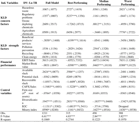
4. RESULTS
Table 1, descriptive statistics, provides means, standard deviations, and ranges for our variables. Table 2, the correlation table, includes all variables in question except for the dummy variable (i.e., industry). Table 3 presents four sets of results: the results of the undifferentiated full population and the CHOW tests for our three heterogeneous environmental performance groups. The model used in each of the four regressions is identical except for the sample size. Note that TR is the dependent variable, a proxy for inverse EP; that is, a larger TR indicates worse EP, whereas a smaller TR indicates better EP.
First, the full population model in column 3 is representative of the common practice in environmental sustainability studies. The next three columns are the heterogeneity tests – the real focus of this research – and represent a step that contributes to the literature. The different patterns of the significant results of the CHOW test across the three differently performing peer groups make clear that we accept our hypotheses about heterogeneity. Clearly, the effects of heterogeneity are substantial across the peer groups at a significant level of the model (i.e., F-value). The implication of these results is that, with respect to environmental policy, one policy for all industries is unlikely to be effective.
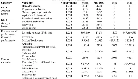
Table 1: Descriptive Statistics
Category Variables Observations Mean Std. Dev. Min Max
KLD concern factors
Hazardous waste 1,231 .4143 .4928 0 1
Regulatory problems 1,231 .4362 .4961 0 1
Ozone depleting chemicals 1,231 .0390 .1937 0 1
Agricultural chemicals 1,231 .0967 .2956 0 1
KLD strength factors
Beneficial products/services 1,231 .1552 .3622 0 1
Pollution prevention 1,231 .1243 .3300 0 1
Recycling 1,231 .1113 .3146 0 1
Clean energy 1,231 .0861 .2806 0 1
Environmental
performance Ln toxic releases (Unit: lbs) 1,231 505,149 17.53 14.99 567,669,533 Financial
performance
EBIT/Sales 1,231 .1125 .0829 –.2772 .5750
Market/Book value 1,231 3.3602 7.5982 –105.221 110.942
Control variables
Available
(current asset/current liabilities) 1,231 1.6014 .7794 .3852 16.7814 Potential
(debt/equity) 1,231 1.2136 2.2536 .0022 37.1926
Recoverable
(SGA/Sales) 1,220 .1673 .1233 .0033 .6431
Firm size (Unit: million dollars
in assets) 1,231 5,874.5 3.72 178 304,592.5
Diversification 1,231 2.6872 1.8890 1 11
CAPX/Sales 1,231 .0792 .1221 .0067 1.9988
Misery index
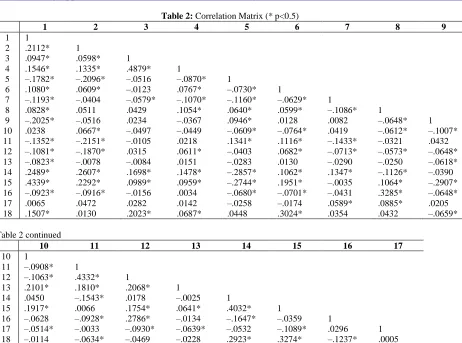
Table 2: Correlation Matrix (* p<0.5)
1 2 3 4 5 6 7 8 9
1 1
2 .2112* 1
3 .0947* .0598* 1
4 .1546* .1335* .4879* 1
5 –.1782* –.2096* –.0516 –.0870* 1
6 .1080* .0609* –.0123 .0767* –.0730* 1
7 –.1193* –.0404 –.0579* –.1070* –.1160* –.0629* 1
8 .0828* .0511 .0429 .1054* .0640* .0599* –.1086* 1
9 –.2025* –.0516 .0234 –.0367 .0946* .0128 .0082 –.0648* 1 10 .0238 .0667* –.0497 –.0449 –.0609* –.0764* .0419 –.0612* –.1007* 11 –.1352* –.2151* –.0105 .0218 .1341* .1116* –.1433* –.0321 .0432 12 –.1081* –.1870* .0315 .0611* –.0403 .0682* –.0713* –.0573* –.0648* 13 –.0823* –.0078 –.0084 .0151 –.0283 .0130 –.0290 –.0250 –.0618* 14 .2489* .2607* .1698* .1478* –.2857* .1062* .1347* –.1126* –.0390 15 .4339* .2292* .0989* .0959* –.2744* .1951* –.0035 .1064* –.2907* 16 –.0923* –.0916* –.0156 .0034 –.0680* –.0701* –.0431 .3285* –.0648* 17 .0065 .0472 .0282 .0142 –.0258 –.0174 .0589* .0885* .0205 18 .1507* .0130 .2023* .0687* .0448 .3024* .0354 .0432 –.0659*
Table 2 continued
10 11 12 13 14 15 16 17
10 1
11 –.0908* 1
12 –.1063* .4332* 1
13 .2101* .1810* .2068* 1
14 .0450 –.1543* .0178 –.0025 1
15 .1917* .0066 .1754* .0641* .4032* 1
16 –.0628 –.0928* .2786* –.0134 –.1647* –.0359 1
17 –.0514* –.0033 –.0930* –.0639* –.0532 –.1089* .0296 1 18 –.0114 –.0634* –.0469 –.0228 .2923* .3274* –.1237* .0005
Table 3: Heterogeneity Test
Ind. Variables DV: Ln TR Full Model Best Performing Median
Performing Worst Performing KLD concern factors Hazardous
waste .1067 (.1077) .2727
† (.1419) .0361 (.1248) .2621† (.1474)
Regulatory
problems .1357 †
(.0807) .5237***(.1356) .1161 (.0915) –.0447 (.1174)
Ozone depleting chemicals
.2609 (.3517) –1.7262 (.8715) .8812** (.3151) –.4959 (.3790)
Agriculture
chemicals .0509 (.1913) .0458 (.2977) –.3460 (.1895) .7776* (.2722)
KLD strength factors
Beneficial products/ services
–.3030* (.1468) –.6199***(.1614) –.0541 (.1488) –.3456 (.3005)
Pollution
prevention .1536 (.1136) –.2029 (.1626) .2544
† (.1328) –.1184 (.1648)
Recycling –.0040 (.1754) .2551 (.2339) –.0925 (.2134) –.0777 (.1972) Clean energy .0439 (.1414) .1188 (.1779) –.0204 (.1570) .3316 (.2840)
Financial performance
EBIT/Sales .5613 (.6123) –.6552(.7332) .6672 (1.0434) .7631 (1.1200) Market/Book
value –.0031 (.0047) –.0390*** (.0095) .0465*** (.0110) .0388**(.0125)
Control variables
Available
slack .2624**(.0877) .3506** (.1257) –.2709 †
(.1503) –.2481 (.1680)
Potential slack –.0362 (.0609) .0269 (.0879) –.0416 (.1011) –.2488*(.1234) Recoverable
slack –1.0557 (.7834) –1.4409 †
(.8520) –1.1590 (.7687) –.4011 (.9945)
CAPX/Sales –1.5483**(.4401) –1.3228** (.4087) 1.3682 (.9785) –.1609 (.8151) Firm size
(4th root of assets)
–.0764* (.0358) .1022** (.0375) .0169 (.0333) –.0363 (.0540)
Diversificatio
n .1947*** (.0511) .2831***(.0560) –.1837***(.0460) –.1342*(.0578) B2C –1.1311* (.5302) –1.6815***(.5411) –.3714(.3798) Dropped Misery index .0590* (.0240) –.1161*(.0432) .1627** (.0516) .1436** (.0538)
Obs. 1211 315 496 388
F-Value 6.61*** 4.83*** 2.84*** 3.82***
R-square 0.1069 0.2744 0.1223 0.1970
* p< 0.05; ** p< 0.01; *** p<0.001; † p<0.1; the result of the separate model including only total concern and strength scores will be provided on request. Numbers in parentheses are the “standard error.”
With respect to the results for the individual ES proxies1 and FP in the three EP groups, a variety of significant results was observed across heterogeneous groups. With respect to both “Beneficial products and services” as a proxy for proactive ES and “Regulatory problems” as a proxy for reactive ES, and for many of the control variables, the results of the full population model are more similar to the results of the BEP group. Nonetheless, we still observe heterogeneity across differently performing peer groups.
By starting with the individual KLD concerns, we interpret the group results that focus on a single independent variable at a time to explain the heterogeneous effects of ES and FP on EP. First, a larger variety of
1
significant concerns exists across the three heterogeneous groups than in the full population. For example, “hazardous waste” is of no importance in the full model but is marginally significant and positive for both the BEP and WEP groups as expected, implying that more waste leads to poor EP.
“Regulatory problems” is significant only for the full model and the BEP group. Therefore, firms with better EP experience have fewer regulatory problems; that is, firms in the BEP group emit smaller TR than those in the counterpart peer groups. That this statement is not true for the MEP and WEP groups given their demonstrably weaker EP is surprising. That “Regulatory problems” for these two groups has no significant coefficients may be the result of the absolute level of their EP being so weak that new regulatory problems have no differential effects in these peer groups.
“Ozone depleting chemicals” and “Agricultural chemicals” are each significant and positive for the MEP group but not for the other peer groups. “Agricultural chemicals” are positively significant only in the WEP group. These results may be characteristic of the industries represented, which represent particular policy problems for regulators.
We turn to individual strength factors. The results show that little variety exists across heterogeneous peer groups. “Beneficial products and services” is negatively significant for the full sample and for the BEP group. Ceteris paribus, because of its negative coefficient, BPS appears to offset the positively signed significant concern, “Regulatory problems,” for that peer group. The marginal effect of BPS is larger in the BEP group than in the full sample model. This result confirms the potential power of proactive environmentally friendly innovation championed by Porter and van der Linde (1995) and Hart and Ahuja (1996) for the best environmentally performing companies.
However, other strength factors are not significant in either the full model or any of the three heterogeneous groups. To our surprise, a marginal but odd positive coefficient exists for “Pollution prevention” for the MEP group, which is contrary to our expectations. This odd result may be explained from the correlation results. Although concern factors are positively correlated with one another (i.e., they show the expected consistent sign), strength factors are positively and negatively correlated with one another. This finding suggests that, compared with the relationships among concern factors, strength factors assumably contradict one another, indicating that the effect of individual ES on EP may be insignificant and less consistent across heterogeneous groups. This result probably warrants further research to overcome the basic limitation of KLD binary data.
The results for the two financial performance variables are very interesting, in part because many hope to prove “doing good by doing well.” First, Table 3 clearly shows that no significant correlation exists between TR and EBIT/Sales, a result that contradicts expectations but that is robust given that it is true for each of the three groups. At least in the industries studied in this paper, we may conclude that the state-of-the-art with respect to TR management is advanced enough that no immediate earnings are incurred in attempting to manage TR levels. In practice, after the EPA was established under Nixon in 1970, the United States has been paying attention to better TR management for a long time. The EPA has made efforts to improve air quality, and it announced in its 2010 report that air pollutants declined by approximately 41% between 1990 and 2010.
Unlike the absence of significant results with respect to short-term FP, the long-run FP, market/book value, has good and bad results. Market value is the “price per share” at year-end and is compared with the year-end book value. Price is volatile. However, because our study period was curtailed in 2005, it is not largely affected by the financial crises of the post-2007 era, slightly facilitating interpretation.
why we cannot ignore a study of group heterogeneity because the full model may mask the hidden true meaning of subgroups.
Practically, these results also lead to an important corporate and public policy issue. In other words, public policy makers and NGO leaders in particular may find these last results disturbing because they point to a divorce of a large sector of the polluting industries in the United States from well-intentioned efforts to create an environmentally sustainable industrial base. For the MEP and WEP groups—perhaps more likely to be “Ozone depleting chemicals” or “Agricultural chemicals” manufacturers—the positive correlation between long-run financial benefit and effective TR signals that efforts to improve EP and reduce TR are very likely worse and are judged by the capital markets as wasteful. For these groups, a higher market-to-book value is correlated with larger TR (i.e., poor EP). For emphasis, we note that the capital market seems to recognize that persisting with or accepting poor EP is a legitimate financially rewarding strategy for companies in these peer groups.
Our results for the MEP and WEP groups point to a policy failure, possibly at the EPA in past years, because the strategies pursued by the agency appear to work only with the best and not with the rest.
We turn to the control variables to complete this discussion. The results show that the control variables are remarkably replete with significant coefficients. First, CAPX clearly has a significant negative effect on TR in the BEP group, although the effect on the margin is slightly smaller than in the full model. That is, compared with MEP and WEP groups, the BEP group may be boosting its TR performance as it expands and renews its plants. As Hart and Ahuja (1996) argued, advancing technology may still contribute to both enhanced productivity (its primary or motivating casus belli) and better EP. Again, the MEP peer group apparently has not been as successful in killing two birds with one stone.
Firm size has a positive effect on TR only in the BEP group. This result points to a need to carefully evaluate the effectiveness of present day public policies across industries for which size itself is one of the variables of interest. The correlations identified for the BEP peer group suggest that large firms may be dragging their feet with respect to improving EP. Diversification has similar results with respect to TR in the BEP group as in the full model, but is negatively correlated with TR for both the MEP and the WEP groups.
We included three types of slack variables. The result shows that available slack is significantly correlated with TR. However, the positive relationship implies that having available (idle) resources may be dysfunctional for the BEP group (and in the full model). The marginal effect for the BEP group is considerably greater than for the full model probably because of the masking effect of the other two groups in the control population. The negative and significant results for potential slack for the WEP group offer some hope for policy makers looking for ways to encourage better EP, to enforce corporate efforts, or at least whom to audit carefully. The results suggest a further need for discrimination at a public policy level when dealing with rules and enforcement for firms in the WEP group. Firms with substantial potential slack may be proving more capable and willing to enhance their TR performance than their financially more conservative peers. Firms not using their debt capacity appear to be the laggards.
B2C is significant and negative in the full model and only for the BEP group of subgroups, another result that supports our contention that heterogeneity matters. Note that a study of the full sample masks the real effects within these industries. Also interesting is the set of results associated with the Misery index in Table 3, which seems to show that, from 1991 to 2005, only the BEP group had the capability to weather the tough high misery years and reduce its TR impacts.
5. DISCUSSION
cross-sectional panel data encompassing three databases. Moreover, we were able to carefully control for several firm attributes, industry, and government administration periods.
To compare the recently recommended method with the common practice (i.e., total scores) for using KLD factors, this study employed individual KLD factors. As previously mentioned, total concern and strength scores may not be valid measures because they are orthogonally correlated with one another. The heterogeneity test provides evidence for the argument that simply aggregating orthogonal factors may mask the hidden true meanings in subgroups and then mislead to confuse the results (Mattingly and Berman, 2006). In contrast, the results for the individual KLD measures are informing and, in some instances, encouraging for policy makers. For example, the particular ES measures, either reactive or proactive, are at least generally consistent with the theory for the BEP group, although mostly inconsistent with the theory for the rest.
Low correlations between KLD concern and strength factors suggest that researchers need to be careful in attributing significant weight to the effects of the sums of total concerns or strengths on EP (Mattingly and Berman, 2006; Chatterji et al, 2009). Our heterogeneity test also suggests that caution is warranted when researchers use separate KLD concerns and strengths as ES proxies unless they confirmed that the sample used is homogeneous. Specifically, the CHOW tests show that recognized heterogeneity gives us the opportunity to more closely appreciate the effects of ES and FP on EP within an industry population. These results also suggest a more exact appreciation of the impacts and failures of TR management, both corporately and publically through regulation and its enforcement. These matters are of considerable importance in a world in which environmental concerns are being translated into legislation.
Generally, this study’s results for the BEP group were more consistent with prior research than those for either the MEP or the WEP peer groups. A possible explanation to consider for a moment is that firms in an environmentally better performing group are more likely to report their ES and EP exactly to the TRI record keepers than firms in environmentally worse or moderately performing groups. However, the different signs and sizes of the coefficients for the control factors in every group argue against this proposition. Perhaps, over time, improved and wider scoped data collection practices at KLD will assist in resolving these questions.
Our results may have additional implications. According to “neoinstitutional theory,” firms imitate what they see in similar firms’ traits and outcomes (Haveman, 1993; Lee and Pennings, 2002). Firms tend to adopt practices or structures adopted by leading firms (Haunschild and Miner, 1997) and tend to imitate other firms in their industry that are perceived as successful (Burns and Wholey, 1993). Firms are always interested in best practices among their peers; therefore, determining the firms to imitate matters. Our results suggest that, with respect to EP and efforts to improve their own EP, firms need to learn how to constructively discriminate—they need to understand the groups in which they belong and the effects of alternate strategies on the particular EP they seek to effect.
6. CONCLUSION
AUTHOR INFORMATION
Kyungho Kim is an assistant professor at School of Business, Ajou University. He received his DBA from Boston University. His research areas include corporate strategy, international business strategy, corporate social responsibility, and environmental sustainability. Kyungho Kim, School of Business, Ajou University, San 5, Woncheon-dong, Yeongtong-gu, Suwon, 443-749, South Korea. E-mail: [email protected]
Hyunwoo Lim is an assistant professor at School of Business, Ajou University. He received his PhD in Management from University of Toronto. His research areas include marketing strategy, econometric modeling, and international marketing. This work was supported by the new faculty research fund of Ajou University. Hyunwoo Lim, School of Business, Ajou University, San 5, Woncheon-dong, Yeongtong-gu, Suwon, 443-749, South Korea. E-mail: [email protected] (Corresponding author)
REFERENCES
1. Allison, P.D. (1984). Event History Analysis: Regression for Longitudinal Event Data. SAGE: Newbury Park, CA.
2. Ambec, S., Lanoie, P. (2008). Does it pay to be green? A systematic overview. The Academy of Management Perspectives (formerly The Academy of Management Executive, AMP), 22(4), 45-62. 3. Berman, S.L., Wicks, A.C., Kotha, S., Jones, T.M. (1999). Does stakeholder orientation matter? The
relationship between stakeholder management models and firm financial performance. Academy of Management Journal, 42(5), 488-506.
4. Bourgeois, L.J. (1981). On the measurement of organizational slack. Academy of Management Review, 6(1), 29-39.
5. Bourgeois, L.J., Singh, J.V. (1983). Organizational Slack and Political Behavior Within Top Management Groups. Faculty of Management Studies, University of Toronto.
6. Bowen, F.E. (2002). Does size matter? Business & Society, 41(1), 118-124.
7. Bromiley, P. (1991). Testing a causal model of corporate risk taking and performance. Academy of Management Journal, 34(1), 37-59.
8. Burns, L.R., Wholey, D.R. (1993). Adoption and abandonment of matrix management programs: Effects of organizational characteristics and interorganizational networks. Academy of management journal, 36(1), 106-138.
9. Buysse, K., Verbeke, A. (2003). Proactive environmental strategies: a stakeholder management perspective. Strategic Management Journal, 24(5), 453-470.
10. Cameron, A.C., Trivedi, P.K. (2009). Microeconometrics Using Stata. Stata Press.
11. Caves, R.E., Porter, M.E., Spence, A.M. 1980. Competition In The Open Economy: A Model Applied to Canada. Harvard Economic Studies.
12. Chatterji, A.K., Levine, D.I., Toffel, M.W. (2009), How well do social ratings actually measure corporate social responsibility? Journal of Economics & Management Strategy, 18(1), 125-169.
13. Chow, G.C. (1960). Tests of equality between subsets of coefficients in two linear regressions. Econometrica, 28(3), 591-605.
14. Dahlmann, F. (2009). Oil Prices & Greening: Antecedents of Evolving Corporate Environmental Strategy in th US. Academy of Management Annual Meeting, Chicago, IL, USA.
15. Delmas, M.A., Blass, V.D. (2010). Measuring corporate environmental performance: The trade-offs of sustainability ratings. Business Strategy and the Environment, 19(4), 245-260.
16. Dixon-Fowler, H.R., Slater, D.J., Johnson, J.L., Ellstrand, A.E. (2009). Beyond "Does it pay to be green?" A Meta-Analysis of Moderators of the CEP and CFP relationship. Academy of Management Annual Meeting, Chicago, IL, USA.
17. Fernando, C., Sharfman, M.P., Uysal, V. (2009). Do investors want firms to be green? Environmental performance, ownership and stock market liquidity. Academy of Management Annual Meeting, Chicago, IL, USA.
18. Fogler, H.R., Nutt, F. (1975). A note on social responsibility and stock valuation. Academy of Management Journal, 18(1), 155-160.
20. Freedman, M., Jaggi, B. (1994). Analysis of the association between pollution performance and input cost factors: The case of electric utility plants. Journal of Accounting and Public Policy, 13(1), 31-48.
21. Friedman, M. (1970). The social responsibility of business is to increase its profits. New York Times Magazine, 32(13), 122-126.
22. Greer, J., Bruno, K. (1996). Greenwash: The reality behind corporate environmentalism. New York: Apex Press.
23. Hart, S.L. (1995). A natural-resource-based view of the firm. Academy of Management Review, 20(4), 986-1014.
24. Hart, S.L., Ahuja, G. (1996). Does it pay to be green? An empirical examination of the relationship between pollution prevention and firm performance. Business Strategy and the Environment, 5(1), 30-37. 25. Hart, S.L., Dowell, G. (2011). Invited Editorial: A natural-resource-based view of the firm. Journal of
Management, 37(5), 1464-1479.
26. Haunschild, P.R., Miner, A.S. (1997). Modes of interorganizational imitation: The effects of outcome salience and uncertainty. Administrative Science Quarterly, 42(3), 472-500.
27. Haveman, H.A. (1993). Follow the leader: Mimetic isomorphism and entry into new markets. Administrative Science Quarterly, 38(4), 593-627.
28. Henriques, I., Sadorsky, P. (1999). The relationship between environmental commitment and managerial perceptions of stakeholder importance. Academy of Management Journal, 42(1), 87-99.
29. Hillman, A.J., Keim, G.D. (2001). Shareholder value, stakeholder management, and social issues: what's the bottom line? Strategic Management Journal, 22(2), 125-139.
30. Hunt, C.B., Auster, E.R. (1990). Proactive environmental management: avoiding the toxic trap. Sloan Management Review, 31(2), 7-18.
31. Judge, W.Q., Douglas, T.J. (1998). Performance implications of incorporating natural environmental issues into the strategic planning process: an empirical assessment, Journal of Management Studies, 35(2), 241-262.
32. Klassen, R.D., McLaughlin, C.P. (1996). The impact of environmental management on firm performance. Management Science, 42(8), 1199-1214.
33. Lee, K., Pennings, J.M. (2002). Mimicry and the market: Adoption of a new organizational form. Academy of Management Journal, 45(1), 144-162.
34. Lo, A.W., Newey, W.K. (1983). A large-sample chow test for the linear simultaneous equation. Economics Letters, 18(4), 351-353.
35. Lothe, S., Myrtveit, I., Trapani, T. (1999). Compensation systems for improving environmental performance. Business Strategy and the Environment, 8(6), 313-321.
36. Lyon, T.P., Van Hoff, B.J. (2009). Evaluating Mexico's green supply chains program. Academy of Management Annual Meeting, Chicago, IL, USA.
37. Margolis, J.D., Elfenbein, H.A., Walsh, J.P. (2007). Does it pay to be good? A meta-analysis and redirection of research on the relationship between corporate social and financial performance. Working paper, Ann Arbor, University of Michigan, 1001: 48109-41234.
38. Mattingly, J.E., Berman, S.L. (2006). Measurement of Corporate Social Action. Business & Society, 45(1), 20-46.
39. McGuire, J.B., Sundgren, A., Schneeweis, T. (1988). Corporate social responsibility and firm financial performance. Academy of Management Journal, 31(4), 854-872.
40. McWilliams, A., Siegel, D. (2000). Corporate social responsibility and financial performance: correlation or misspecification? Strategic Management Journal, 21(5), 603-609.
41. Mitchell, R.K., Agle, B.R., Wood, D.J. (1997). Toward a theory of stakeholder identification and salience: Defining the principle of who and what really counts. Academy of Management Review, 22(4), 853-886. 42. Nehrt, C. (1998). Maintainability of first mover advantages when environmental regulations differ between
countries. Academy of Management Review, 23(1), 77-97.
43. Orlitzky, M., Schmidt, F.L., Rynes, S.L. (2003). Corporate social and financial performance: A meta-analysis. Organization Studies, 24(3), 403-441.
44. Pogutz, S., Russo, A. (2009). Eco-efficiency vs. Eco-effectiveness: Exploring the link between GHG emissions and firm performance. Academy of Management Annual Meeting, Chicago, IL, USA.
46. Porter, T.B. (2006). Coevolution as a research framework for organizations and the natural environment. Organization & Environment, 19(4), 479-504.
47. Post, J.E., Preston, L.E., Sauter-Sachs, S. (2002). Redefining the corporation: Stakeholder management and organizational wealth. Stanford University Press.
48. Rehbein, K., Waddock, S., Graves, S.B. (2004). Understanding shareholder activism: Which corporations are targeted? Business & Society, 43(3), 239-267.
49. Russo, M.V., Fouts, P.A. (1997). A resource-based perspective on corporate environmental performance and profitability. Academy of Management Journal, 40(3), 534-559.
50. Sharma, D.S. (2002). The differential effect of environmental dimensionality, size, and structure on budget system characteristics in hotels. Management Accounting Research, 13(1), 101-130.
51. Sharma, S., Vredenburg, H. (1998). Proactive corporate environmental strategy and the development of competitively valuable organizational capabilities. Strategic Management Journal, 19(8), 729-753.
52. Sharma, S. (2000). Managerial interpretations and organizational context as predictors of corporate choice of environmental strategy. Academy of Management Journal, 43(4), 681-697.
53. Sharma, S., Henriques, I. (2005). Stakeholder influences on sustainability practices in the Canadian forest products industry. Strategic Management Journal, 26(2), 159-180.
54. Strike, V.M., Gao, J., Bansal, P. (2006). Being good while being bad: social responsibility and the international diversification of US firms. Journal of International Business Studies, 37(6), 850-862. 55. Waddock, S.A., Graves, S.B. (1997). The corporate social performance-financial performance link.
Strategic Management Journal, 18(4), 303-319.
56. Walley, N., Whitehead, B. (1994). It's not easy being green. Harvard Business Review, 72(3), 46-52. 57. Wernerfelt, B., Montgomery, C.A. (1988). Tobin's q and the importance of focus in firm performance. The