Grouped Bees Algorithm: A Grouped Version of the Bees Algorithm

Article

Grouped Bees Algorithm: A Grouped Version of the

Bees Algorithm

Hamid Reza Nasrinpour 1_{, Amir Massah Bavani} 2,_{* and Mohammad Teshnehlab} 3

1 _{Electrical and Computer Engineering Department, University of Manitoba, Winnipeg, MB R3T 2N2,} Canada; [email protected]

2 _{Electrical and Computer Engineering Faculty, Technical University of Kaiserslautern, Kaiserslautern 67663,} Germany

3 _{Electrical and Computer Engineering Faculty, K.N. Toosi University of Technology, Tehran 19697 64499,} Iran; [email protected]

* Correspondence: [email protected]; Tel.: +49-152-38937661

Abstract: As with many of the non-deterministic search algorithms, particularly those are analogous to complex biological systems, there are a number of inherent difficulties, and the Bees Algorithm (BA) is no exception. Basic versions and variations of the BA have their own drawbacks. Some of these drawbacks are a large number of parameters to be set, lack of methodology for parameter setting and computational complexity. This paper describes a Grouped version of the Bees Algorithm (GBA) addressing these issues. Unlike its conventional version, in this algorithm bees are grouped to search different sites with different neighbourhood sizes rather than just discovering two types of sites, namely elite and selected. Following a description of the GBA, the results gained for 12 benchmark functions are presented and compared with those of the basic BA, enhanced BA, standard BA and modified BA to demonstrate the efficacy of the proposed algorithm. Compared to the conventional implementations of the BA, the proposed version requires setting of fewer parameters, while producing the optimum solutions much faster.

Keywords: bees algorithm; swarm intelligence; evolutionary optimization; grouped bees algorithm

1. Introduction

In recent years, we have considered many applications of population-based search algorithms in a diverse area of both theoretical and practical problems. Basically, these heuristic searches algorithms are exceedingly well suited for optimization problems by huge number of variables. Due to the nature of these multi variable problems, it is almost impossible to find a precise solution set for them within a polynomial bounded computation time. Therefore, swarm-based algorithms are preferred for finding the most optimal solution as much as possible within a sensible time. A number of most well-known stochastic optimization methods are (but are not limited to) Ant Colony Optimization (ACO) [1], Artificial Bee Colony (ABC) algorithms [2], Genetic Algorithms (GA) [3], Particle Swarm Optimization (PSO) [4], Cuckoo Search (CS) algorithm [5] and the Bees Algorithm (BA) [6].

The ACO algorithm mimics real ants’ behaviour in seeking food. Real ants generally wander arbitrarily to find food, and once it was found, they return to their colony while making a trail by spreading pheromone. If other ants face such a path, they will follow and reinforce the track, or revise it in some cases. Some theoretical and practical application of ACO can be found in [7, 8]. Some improvements for the search mechanism of ACO using derivative free optimization methods can be found in [9].

bees: employed, onlooker and scout. In the ABC, the employed bees are responsible to look for new food resources affluent of nutrient within the vicinity of the food resources that they have visited before [10]. Onlookers monitor the employed bees’ dancing and choose food resources based on the dances. Finally, the task of finding new food resources in a random manner is given to scout bees. The performance of ABC versus GA and PSO has been evaluated by testing them on a set of multi variable optimization problems in [11]. An example of the ABC application to increase throughput for wireless sensor networks is given in [12].

The GA and PSO are two other well-known optimization algorithms which are inspired from two different biological approaches. The former works according to the evolutionary idea of the natural selection and genetics; and the latter imitate the “social behaviour of bird flocking or fish schooling” [13]. The two techniques have been applied in a vast number of applications. As an example, the performance of ACO, PSO, and GA on the radio frequency magnetron sputtering process is compared in [14]. A recent variant of the GA known as “Quantum Genetic Algorithm” is reviewed in [15].

The CS, another meta-heuristic search algorithm, is introduced by Yang and Deb in 2009 [5]. This algorithm imitates the “obligate brood parasitic behaviour” of some cuckoos which put their eggs in nests of other birds [16]. A solution is represented by an egg which can be found by another host bird by a specific likelihood. The host bird can then follow two policies: to toss the egg out, or to drop the nest in order to construct a new nest. As such, the highest quality nest will be transferred through the generations to keep the best solutions over the process. A review on the CS algorithm and its application can be find in [17]. A conceptual comparison of the CS to ABC and PSO can be found in [18].

The BA is another optimization algorithm derived from the food seeking behaviour of honey bees in nature. A detailed description of BA can be found in section 4. A comprehensive survey and comparison of BA to ABC and PSO is presented in [19]. The basic BA and its other versions have been widely used in various problems including manufacturing cell formation [20], integer-valued optimizations for designing a gearbox [21], printed-circuit board (PCB) assembly configuration [22], [23], machine job scheduling [24], adjusting membership functions of a fuzzy control system [25], neural network training [26], data clustering [27], automated quiz creator system [28], and for channel estimation within a MC-CDMA (Multi-Carrier Code Division Multiple Access) communication system [29].

In the literature, various versions of BA such as enhanced BA, standard BA and modified BA have been introduced after the introduction of the basic BA. Reference [30] gives a fairly detailed review of many different versions of BA. The enhanced BA has higher computational complexity because of its included fuzzy subsystem which selects potentially better sites or patches (i.e. solutions) for better exploration, albeit it is reducing the number of setting parameters. The standard BA has increased the accuracy and speed by applying two new procedures on the basic version. This improvement has led to higher complexity for standard BA. In the modified BA, a collection of new operators is added to the basic BA which results in performance improvement, and consequently, too much increasing of complexity compared to all the other versions.

2. Results

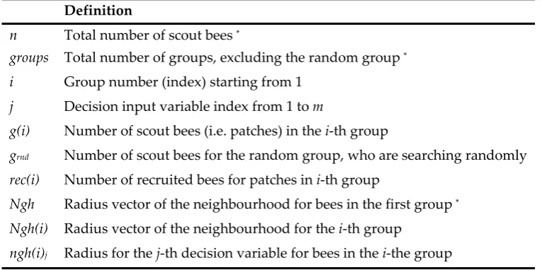
In order to access the performance (i.e. speed and accuracy) of the proposed GBA, the algorithm was applied on 12 well-known function benchmarks. The results are then compared to those reported in [6], [31], [32].

2.1. Benchmark set

For each function, the interval of the input variables, the equation and the global optimum are shown in Table 1 as reported in [33], [34].The Martin & Gaddy and Hypersphere benchmarks are uni-modal functions which are quite straightforward for optimization tasks. The Branin function has three global optima with exact the same value. The minimum of the unimodal Rosenbrock function is at the lowest part of a long and narrow valley [19]. While the valley could be simply discovered within a few repetitions of the optimization algorithm, locating the exact global minimum is quite difficult. The Goldstein & Price function is also an easy benchmark for optimization with only two input parameters. The Schwefel function is quite misleading where the global minimum is in distant from the second best minimum [33]. As such, the optimization algorithms could easily fall into the trapped second best minimum. The multi-modal Shekel function has a complex search space. The Steps benchmark is formed of many flat plateaus and steep ridges. The Griewangk and Rastrigin functions are extremely multi-modal. Both functions include a cosine modulation creating numerous local minima. Yet the locations of the local minima throughout the search space are regularly spread [33].

2.2. Speed evaluation

As the first experiment, the proposed algorithm was tested for speed, and compared to the basic BA [6] and the enhanced BA on the benchmark functions from 1 to 7. The experiment conditions were set according to the experiments of Pham and his colleagues [19], [31]. Accordingly, the grouped Bees Algorithm was run 100 times, with different random initializations, for each of these functions. The error for the while-loop of the GBA was defined as the difference between the value of the global optimum and the fittest solution found by the GBA, so far. The optimization procedure then stopped when the error was less than the minimum of 0.001 and 0.1% of the global optimum. When the optimum value was zero, the procedure stopped if the solution was different from the optimum value by less than 0.001. From mathematical perspective, the stopping criteria were hence set to be:

= ( ) − ∗ _(2.1)

= ≤ 0.001 ; ( ) = 0

≤ 0.001, 0.1

100 ( ) ; ( ) ≠ 0

(2.2)

where f(x) is the value of the benchmark function f at the input point of x, and f* is the value of its global optimum.

Table 2. Mean number of evaluations of functions 1-7 for BA, EBA [31] and GBA.

Function Mean number of Evaluations

Basic BA Enhanced BA Grouped BA

1. Martin & Gaddy 2D 526 124 114

2. Branin 3D 1657 184 216

3. Rosenbrock 4D 28529 33367 29601

4. Hypersphere 6D 7113 526 565

5a. Rosenbrock 2D 2306 1448 1026

5b. Rosenbrock 2D 631 689 580

5c. Rosenbrock 2D 868 830 679

6. Goldstein & Price 2D 999 212 273

7. Schwefel 6D Approx. 3E6 N/A Approx. 1E6

Table 3. Differences in the average number of evaluations.

Function Percentage Change in GBA w.r.t.

Basic BA Enhanced BA

1. Martin & Gaddy 2D -78.33% -8.06%

2. Branin 3D -86.96% 17.39%

3. Rosenbrock 4D 3.76% -11.29%

4. Hypersphere 6D -92.06% 7.41%

5a. Rosenbrock 2D -55.51% -29.14%

5b. Rosenbrock 2D -8.08% -15.82%

5c. Rosenbrock 2D -21.77% -18.19%

6. Goldstein & Price 2D -72.67% 28.77%

Average -51.45% -3.62%

Table 4. The parameters used by GBA in the speed experiment

Function n groups Ngh*

1. Martin & Gaddy 2D 6 3 0.13

2. Branin 3D 8 3 0.05

3. Rosenbrock 4D 4 3 0.001

4. Hypersphere 6D 4 3 0.035

5a. Rosenbrock 2D 5 3 0.11

5b. Rosenbrock 2D 6 3 0.08

5c. Rosenbrock 2D 4 3 0.09

6. Goldstein & Price 2D 9 3 0.006

7. Schwefel 6D 500 3 0.2

Figure 1. Search Strategy of GBA and EBA [31] on Shekel Function.

2.3. Accuracy evaluation

As the second experiment, the proposed algorithm was tested for accuracy, and compared to the standard BA [19] and the modified BA [32] on the benchmark functions from 5c to 12. The standard BA is a better version of the basic BA which employs neighbourhood shrinking and site abandonmentmethods [19]. The stopping criteria in this experiment are defined differently form the first experiment. The experiment conditions were set according to the experiments in [32]. Hence, the grouped Bees Algorithm was run independently 20 times as was an experiment condition in [32]. By the end of each run, the fittest bee of the last iteration was considered to be the final solution. For each benchmark problem, the exact number of iterations was preset in such a way that the number of function evaluations was as close as possible to that of the standard Bees Algorithm or the modified BA in [32], whichever was smaller. Precisely speaking, equations (2.3) - (2.5) show how to calculate the exact number of iterations and function evaluations in the GBA.

The number of evaluations in one iteration (λ) of GBA is defined as:

= ( ). ( ) + (2.3)

As a result, the number of iterations, , and the number of evaluations, , are obtained as:

= (2.4)

= . (2.5)

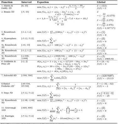
where δ is the minimum number of evaluations in the standard BA and the modified BA. The number of iterations and function evaluations for the three mentioned algorithms are provided in Table 5. The table shows the differences in the number of function evaluations between GBA and the other two algorithms in percentages. The absolute distance from the fitness of the final solution to the global optimum is denoted as the absolute error as is in [32]. Alike to [32], for each algorithm, the average and the median of absolute error are given in Table 6. These numbers are displayed in decimal to an accuracy of 4 decimal places. The least errors obtained for each benchmark function are emphasised in bold. If two algorithms performed similarly, their results are both displayed in bold. Table 7 shows the parameters used by the GBA for benchmark functions from 5c to 12 in the accuracy experiment.

eight benchmarks. Considering both the mean and median errors, the grouped BA and the modified BA have performed almost equally in general. However, the standard BA has an equal or worse performance than the GBA in six benchmark functions out of eight.

Table 5. No. of iterations and evaluations by Grouped BA, Standard BA and Modified BA

Modified BA Standard BA Grouped BA Function Diff.% Iter. Eval. Diff.% Iter. Eval. Iter. Eval. 4.79% 50 503 2.92% 19 494 32 480 5c. Rosenbrock 2D

0.59% 100 1026 1.96% 40 1040 51 1020 6. Goldstein & Price 2D

1.98% 200 2011 1.52% 77 2002 16 1972 7. Schwefel 6D

3.85% 100 1026 5.26% 40 1040 19 988 8. Shekel Foxholes 2D

5% 10 126 8.33% 5 130 8 120 9. Steps 5D

1.38% 100 1026 2.77% 40 1040 11 1012 10. Rosenbrock 5D

0.59% 100 1026 1.96% 40 1040 68 1020 11. Griewangk 10D

1.08% 100 1026 2.46% 40 1040 35 1015 12. Rastrigin 20D

Table 6. Mean and median of absolute error for Grouped BA, Standard BA and Modified BA

Modified BA Standard BA Grouped BA Function Median Mean Median Mean Median Mean 0.0003 0.0014 0.0078 0.0224 0.0002 0.0019

5c. Rosenbrock 2D

0.0000 0.0011 0.0000 0.0000 0.0000 0.0000

6. Goldstein & Price 2D

73.4942 93.0656 572.2723 620.3443 454.0311 453.2246

7. Schwefel 6D

0.0000 0.1525 0.0095 0.0213 0.0000 0.2397

8. Shekel Foxholes 2D

4.0000 3.8500 4.5000 4.2000 2.0000 2.1500

9. Steps 5D

0.8540 1.3038 1.3728 1.2090 1.1019 1.3319

10. Rosenbrock 5D

1.0718 1.0774 1.0887 1.0774 0.9483 0.9297

11. Griewangk 10D

77.8710 83.7651 120.6735 116.2691 79.3220 83.6515

12. Rastrigin 20D

3 3

5 Wins

Table 7. The parameters used by GBA in the accuracy experiment

Function n groups Ngh*

5c. Rosenbrock 2D 4 3 0.2

6. Goldstein & Price 2D 9 3 0.006

7. Schwefel 6D 20 6 0.5

8. Shekel Foxholes 2D 40 2 0.3

9. Steps 5D 4 3 3

10. Rosenbrock 5D 7 6 0.02

11. Griewangk 10D 4 3 10

12. Rastrigin 20D 15 3 0.025

* _{The Ngh vector has the same scalar value in all dimensions}

3. Discussion

the complex modified BA. It is notable that the modified BA is not considered as one of the main implementations of the Bees Algorithm [30]. The modified BA may be considered as a hybrid kind of BA that employs various operators including mutation, crossover, interpolation and extrapolation; whereas the GBA is not introducing any new operator to the basic BA, and has significantly less conceptual and computational complexity compared to all the other variants built on top of the basic BA.

To compare the performance of the Bees Algorithm family with those of other population-based algorithms, like GA, PSO or ACO, see [19], [31], [32]. Nevertheless, it is worth mentioning that, based on these studies, the Bees Algorithm family outperforms all the other population-based algorithms for these kinds of continuous optimization problems.

A further extension of this work focuses on comparing and discussing the performance of GBA against the Genetics Algorithm and Simulated Annealing on optimizing discreet input space and combinatorial problems such as travelling salesman problem and component placement problem, initially discussed in [35].

4. Materials and Methods

4.1 The Bees Algorithm

The Bees Algorithm (BA), which imitates the natural food seeking behaviour of a swarm of honey bees, fits in the category of population-based optimization algorithms. Figure 2 shows the flowchart of the BA [36]. User needs to initialize a number of parameters before the algorithm begins the optimization process. These parameters are known as: the number of scout bees (n), number of selected sites out of n recently visited regions for neighbourhood search (m), number of elite sites out of m selected regions (e), number of recruited bees for the top e sites (nep), number of recruited bees for the remaining (m-e) selected regions (nsp), and finally, the initial size of each site (ngh) [6]. It is needful to state that a site (or patch) represents an area in the search domain that contains the visited spot and its vicinity.

Figure 2. Basic Bees Algorithm flowchart as reported in [36]

4.1.1 Previous modifications to the Bees Algorithm

The large number of parameters which should be set is a downside of the basic Bees Algorithm. Although some variations of the Bees Algorithm attempt to solve this issue, it is reached at the expense of higher computational complexity. In [31] an enhanced version of the BA, employing two features of a fuzzy greedy system for selection of patches and a hierarchical abandonment method, is described. The abandonment method was first introduced by Ghanbarzadeh [38]. When the algorithm is stuck in a local optimum, this method triggers by removing the trapped site from the list of potential sites [38]. A hierarchical version of abandonment executes the same instruction on all sites with a lower rank than the trapped site [31]. The hierarchical version is utilized in the enhanced BA. A list of sorted candidate solutions based on their fitness determines the rank for each site. The Takagi-Sugeno fuzzy selection system decides the number of selected sites and the number of recruited bees for each site based on a greedy policy [31]. This fuzzy inference process needs to be executed in every iteration which may not be a favorable approach in an iterative algorithm.

Setting two parameters, the “number of scout bees” and the “maximum number of recruited bees for each site” are required in the enhanced BA [31]. The two parameters can have same values, and the initial size of the sites’ neighbourhood (nh) is set to be a fraction of the size of the whole search domain. Figure 3 illustrates the pseudo-code of the Enhanced BA (EBA) [31].

For improving the search accuracy and computation performance, two other procedures are introduced [39], [40]. In the first approach, the search begins within the initial neighbourhood size of sites (nh) of basic BA. It counties using the initial neighborhood size as long as the recruited bees are discovering better solutions in the neighbourhood. If the recruited bees fail to make any progress, the size of the patch will become smaller. This procedure is called the “neighbourhood shrinking” method [39]. In [19], the heuristic formula for updating the size of neighbourhood for each input variable is stated as follows:

ℎ( + 1) = 0.8 ℎ( ) (4.2)

where Max and Min indicate the maximum and minimum of the input vector respectively.

Figure 3. Pseudo code of Enhanced Bees Algorithm (EBA) taken from [31]

If shrinking the patch size does not result in any progress, the second procedure is applied. After a given number of loops, the patch is assumed to be trapped within a local minimum (or peak), and no further improvement would occur [19]. Therefore, the patch exploration is stopped and a new random patch is generated for hunting. This process is known as “abandon sites without new information” [40] or “site abandonment” [19], [40].

The basic version of PSO depends on the swarm's best known position, and this feature leads the algorithm to be potentially trapped in a local peak. This is an untimely convergence which can be eluded by including variable size neighbourhood search and random search into the basic PSO algorithm to escape from stagnant states and reach global optimum [41]. In the same current position and local best position case, a PSO particle would only escape from this point if the previous speed and inertia weight of the particle have been non-zero. However, if previous velocities of the particles are around zero, all of them will stop searching when they reach this local peak, and this can lead to an immature convergence of the algorithm. This premature convergence problem of basic PSO is solved by proposing a hybrid version of PSO-BA [41].

A different formulation for the Bees Algorithm is introduced by including new search operators and a new selection procedure which augment the survival probability of newly formed individuals. This improvement enhances random search process of the Bees Algorithm using following operators: mutation, creep, crossover, interpolation and extrapolation [42]. Every bee or solution has a chance for improvement by evolving a few times using the mentioned operators, and generation by generation the best bee is kept. At each step, a new movement will only be accepted if any improvement is obtained, otherwise its current point will be retained. The number of iterations of the main loop is an inverse function of the fitness rank of the solution. This improved version strongly preserves the best bees. In addition, it keeps creating fresh bees and fostering them. Therefore, the large set of “best bees” would be resumed to search again if they need to be [42].

testing it on nine function benchmarks and comparing the results with that of other algorithms including standard BA, PSO, GA and so forth [32]. To the best of authors’ knowledge, MBA has been the strongest version of the Bees Algorithm for single-objective problems to date, yet at the expense of adding many complex operators.

Apart from the basic neighbourhood search method, two more methods are introduced in [43] to cope with multi-objective problems, where the “pareto” curve is formed by “all the non-dominated bees in each iteration”. During a simple neighbourhood hunt, a recruited bee is dispatched to a selected site and its fitness is calculated; and then, its fitness is compared against the scout bee in the site. The old solution is replaced by the new one only if it could reach a fitter point in search space, otherwise it is not. Based on the first approach, all the recruited bees, the number of which is nsp + nep, are sent to the selected site at the same time rather than one bee at a time. Then, the non-dominant bees are selected among the all recruited bees considering their quality. Finally, the new scout bee will be selected for the site randomly, provided that there are at least two non-dominated bees. This approach is called “Random selection neighbourhood search”, and the second approach is named “Weighted sum neighbourhood search,” which is similar to the random one. In spite of that, where the algorithm is deciding to choose the new scout bee by chance, a linear combination of the objective functions decides which “non-dominated bee” should replace the old scout in the site [44].

4.2 The proposed Grouped Bees Algorithm

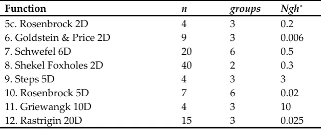
The proposed Grouped Bees Algorithm (GBA) uses the basic Bees Algorithm as a core. The main difference between the basic BA and the grouped BA is the number of different patch types to be explored. This number in the basic BA is two where there are always two types of selected patches, being either elite or good; whereas this number is essentially variable in GBA. In addition, this algorithm, unlike the basic BA, does not waste any patch and searches all of them. In GBA, bees are grouped to search all the patches with different neighbourhood sizes. As such, it is no longer required to set the values of m, e, nep and nsp as the equivalent parameters for each group are determined based on mathematical relations by the algorithm. The GBA has three parameters to be set as: (1) the number of scout bees (n) which corresponds to the total number of patches (or sites) to be explored; (2) the number of strategical searching groups (groups) (3) the patch radiuses for the first group, containing top-rated scout bees, (Ngh). These parameters and some other important notations of GBA are summarized in Table 8.

The algorithm follows three general intuitive rules as follows: (1) while a scout bee is becoming closer to the global optimum, a more precise and detailed exploration is needed; so the search neighbourhood size becomes smaller (for the groups with smaller indices) and vice versa; (2) Based on the nature of honey bees [45], [46], better flower patches, which generally corresponds to groups with smaller indices, should be visited by more recruited bees; (3) The larger neighbourhood size (radius), the more scout bees are needed to cover the whole area.

Similar to the BA mathematical notations [19], the input domain of all possible solutions is considered to be U = {X ∈ℝm_{; Min < X < Max}. So, assuming a fitness function is defined as f(X): U} → R, each potential solution (bee) is formulated as an m-dimensional vector of input variables X = {x1,...,xj,...,xm} where xj is between minj and maxj, corresponding to the decision variable number j. The search neighbourhood for the whole set of bees belonging to the same group of i is defined as an m-dimensional ball with the radius vector of Ngh(i) = {ngh(i)1,... ngh(i)j,...,ngh(i)m} which is centered on the scout bees in the group i. In fact, each (recruited) bee will search on its own neighbourhood (patch), but the neighbourhood size is the same for all bees belonging to the same group. Now, considering the first rule, it is suggested each radius of ngh(i)j should have the following relation with the group number, i:

ℎ( ) = . + (4.3)

ℎ = ℎ(1) = ℎ(1) , . . , ℎ(1) , . . , ℎ(1)

ℎ( ) = −

2

(4.4)

which yields:

=

−

2 − ℎ(1)

− 1

= ℎ(1) −

(4.5)

A simple equation for the number of recruited bees in each group, which is in line with the second rule, is decided to be:

( ) = ( + 1 − )

1 ≤ ≤ (4.6)

Table 8. The Nomenclature of Grouped Bees Algorithm (GBA)

Definition

n Total number of scout bees *

groups Total number of groups, excluding the random group * i Group number (index) starting from 1

j Decision input variable index from 1 to m

g(i) Number of scout bees (i.e. patches) in the i-th group

grnd Number of scout bees for the random group, who are searching randomly rec(i) Number of recruited bees for patches in i-th group

Ngh Radius vector of the neighbourhood for bees in the first group * Ngh(i) Radius vector of the neighbourhood for the i-th group

ngh(i)j Radius for the j-th decision variable for bees in the i-the group * _{To be set by user, whereas other parameters are automatically calculated.}

Given the third rule, it is proposed that the number of scout bees in each group, g(i), should be proportional to the group index square, i2_{, while the total number of all the scout bees who search} either randomly or strategically should be equal to n. To that aim, the area under the graph of k.x2 over the interval [1, groups+1] should sum up to n. So, the problem is to find a coefficient, k, which makes the definite integral of the function of f(x) = k.x2 _{with respect to x from 1 to groups+1 equal to n,} i.e., to find k so as to:

. = (4.7)

which results:

= 3

( + 1) − 1 (4.8)

Given the above, the algorithm determines the number of scout bees in each group as:

( ) = .

( ) = 0 ℎ ( ) = 1 (4.9)

= − ( ) (4.10)

where x+ = max(x, 0); to recapitulate, Figure 4 illustrates the pseudo code of the Grouped Bees Algorithm.

Figure 4. Pseudo code of the Grouped Bees Algorithm (GBA)

5. Conclusions

In this study, the basic version of the Bees Algorithm has been restructured to improve its performance while decreasing the number of setting parameters. The proposed version is denoted as the Grouped Bees Algorithm (i.e. GBA). In contrast to the basic Bees Algorithm, in GBA the bees are grouped to search different patches with various neighbourhood sizes. The group with the lowest index contains the fittest scout bees. This group has also the highest number of recruited bees. As the index of a group increases, the quality of the patches is reduced, and more scout bees are required to discover alternative potential solutions. There is also a random search group with at least one scout bee to preserve the stochastic nature of the algorithm.

The efficiency of the algorithm is assessed with two criteria: converging speed and accuracy. The algorithm is applied on 12 function benchmarks. The net result indicates that the proposed variant is two times faster than the conventional Bees Algorithm, while almost as accurate as the more complex modified BA. Other desirable characteristics of the algorithm can be summarized as follows: (1) The grouped BA (GBA) has a well-defined methodology to set parameters, which leads to a fewer number of tunable parameters; (2) The algorithm entails the least computational load; (3) It is based only on the conventional operators of the Bees Algorithm.

Acknowledgments: The authors thank Professor Robert Donald (Bob) McLeod of the University of Manitoba for his helpful comments and insightful editing.

Author Contributions: Nasrinpour and Massah Bavani conceived and designed the experiments; they performed the experiments, analyzed the result, and wrote the paper. Teshnehlab contributed in design and analysis of the proposed algorithm.

Conflicts of Interest: The authors declare no conflict of interest.

References

1. [1] M. Dorigo and T. Stützle, Ant colony optimization. MIT Press, 2004.

3. [3] D. E. (David E. Goldberg, Genetic algorithms in search, optimization, and machine learning. Addison-Wesley Longman Publishing Co., Inc., 1989.

4. [4] J. Kennedy and R. Eberhart, “Particle swarm optimization,” in Proceedings of ICNN’95 - International Conference on Neural Networks, 1995, vol. 4, pp. 1942–1948.

5. [5] X.-S. Yang and S. Suash Deb, “Cuckoo Search via Lévy flights,” in 2009 World Congress on Nature & Biologically Inspired Computing (NaBIC), 2009, pp. 210–214.

6. [6] D. T. Pham, A. Ghanbarzadeh, E. Koc, S. Otri, S. Rahim, and M. Zaidi, “The Bees Algorithm, A Novel Tool for Complex Optimisation Problems,” in 2nd International Virtual Conference on Intelligent Production Machines and Systems (IPROMS), 2006, pp. 454–459.

7. [7] T. C. Fogarty and I. C. Parmee, Evolutionary computing : AISB Workshop, Sheffield, U.K., April 3-4, 1995 : selected papers. Springer, 1995.

8. [8] M. Mathur, S. B. Karale, S. Priye, V. K. Jayaraman, and B. D. Kulkarni, “Ant Colony Approach to Continuous Function Optimization,” Ind. Eng. Chem. Res., vol. 39, no. 10, pp. 3814–3822, Oct. 2000.

9. [9] F. Rebaudo, V. Crespo-Perez, J.-F. Silvain, and O. Dangles, “Agent-Based Modeling of Human-Induced Spread of Invasive Species in Agricultural Landscapes: Insights from the Potato Moth in Ecuador,” J. Artif. Soc. Soc. Simul., vol. 14, pp. 1–22, 2011.

10. [10] D. Karaboga and B. Basturk, “On the performance of artificial bee colony (ABC) algorithm,” Appl. Soft Comput., vol. 8, no. 1, pp. 687–697, 2008.

11. [11] D. Karaboga and B. Basturk, “A powerful and efficient algorithm for numerical function optimization: artificial bee colony (ABC) algorithm,” J. Glob. Optim., vol. 39, no. 3, pp. 459–471, Oct. 2007. 12. [12] A. Singh and A. Nagaraju, “An Artificial Bee Colony-Based COPE Framework for Wireless Sensor

Network,” Computers, vol. 5, no. 2, p. 8, May 2016.

13. [13] S. Saini, D. R. Bt Awang Rambli, M. N. B. Zakaria, S. Bt Sulaiman, S. Saini, D. R. Bt Awang Rambli, M. N. B. Zakaria, and S. Bt Sulaiman, “A Review on Particle Swarm Optimization Algorithm and Its Variants to Human Motion Tracking,” Math. Probl. Eng., vol. 2014, pp. 1–16, 2014.

14. [14] N. Mohd Sabri, N. Md Sin, M. Puteh, and M. Mahmood, “Optimization of Nano-Process Deposition Parameters Based on Gravitational Search Algorithm,” Computers, vol. 5, no. 2, p. 12, Jun. 2016.

15. [15] R. Lahoz-Beltra and Rafael, “Quantum Genetic Algorithms for Computer Scientists,” Computers, vol. 5, no. 4, p. 24, Oct. 2016.

16. [16] D. N. Vo, P. Schegner, and W. Ongsakul, “Cuckoo search algorithm for non-convex economic dispatch,” IET Gener. Transm. Distrib., vol. 7, no. 6, pp. 645–654, Jun. 2013.

17. [17] A. B. Mohamad, A. M. Zain, and N. E. Nazira Bazin, “Cuckoo Search Algorithm for Optimization Problems—A Literature Review and its Applications,” Appl. Artif. Intell., vol. 28, no. 5, pp. 419–448, May 2014.

18. [18] P. Civicioglu and E. Besdok, “A conceptual comparison of the Cuckoo-search, particle swarm optimization, differential evolution and artificial bee colony algorithms,” Artif. Intell. Rev., vol. 39, no. 4, pp. 315–346, Apr. 2013.

19. [19] D. T. Pham and M. Castellani, “The Bees Algorithm: modelling foraging behaviour to solve continuous optimization problems,” Proc. Inst. Mech. Eng. Part C J. Mech. Eng. Sci., vol. 223, no. 12, pp. 2919–2938, Dec. 2009.

20. [20] D. T. Pham, A. A. Afify, and E. Koç, “Manufacturing cell formation using the Bees Algorithm,” in

Innovative Production Machines and Systems Virtual Conference, 2007.

21. [21] Pham D T, Castellani M, and Ghanbarzadeh A, “Preliminary design using the Bees Algorithm,” in

8th International Conference on Laser Metrology, CMM and Machine Tool Performance, 2007.

22. [22] D. T. Pham, S. Otri, and A. H. Darwish, “Application of the Bees Algorithm to PCB assembly optimisation,” in 3rd Virtual Int. Conf. on Innovative Production Machines and Systems, 2007, pp. 511–516. 23. [23] C. A. Mei, D. T. Pham, J. S. Anthony, and W. N. Kok, “PCB assembly optimisation using the Bees

Algorithm enhanced with TRIZ operators,” in IECON 2010 - 36th Annual Conference on IEEE Industrial Electronics Society, 2010, pp. 2708–2713.

24. [24] D. T. Pham, E. Koç, J. Y. Lee, and J. Phrueksanant, “Using the Bees Algorithm to schedule jobs for a machine,” in 8th international Conference on Laser Metrology, CMM and Machine Tool Performance

(LAMDAMAP), 2007, pp. 430–439.

26. [26] D. . Pham, A. Soroka, A. Ghanbarzadeh, E. Koc, S. Otri, and M. Packianather, “Optimising Neural Networks for Identification of Wood Defects Using the Bees Algorithm,” in 2006 IEEE International Conference on Industrial Informatics, 2006, pp. 1346–1351.

27. [27] H. Al-Jabbouli, Data clustering using the Bees Algorithm and the Kd-Tree structure: Flexible data

management strategies to improve the performance of some clustering algorithms. LAP Lambert Academic

Publishing, 2011.

28. [28] P. Songmuang and M. Ueno, “Bees Algorithm for Construction of Multiple Test Forms in E-Testing,”

IEEE Trans. Learn. Technol., vol. 4, no. 3, pp. 209–221, Jul. 2011.

29. [29] F. Sayadi, M. Ismail, N. Misran, and K. Jumari, “Multi-Objective optimization using the Bees algorithm in time-varying channel for MIMO MC-CDMA systems,” Eur. J. Sci. Res., vol. 33, no. 3, pp. 411– 428, 2009.

30. [30] W. A. Hussein, S. Sahran, and S. N. H. Sheikh Abdullah, “The variants of the Bees Algorithm (BA): a survey,” Artif. Intell. Rev., pp. 1–55, Apr. 2016.

31. [31] D. T. Pham and A. H. Darwish, “Fuzzy Selection of Local Search Sites in the Bees Algorithm,” in 4th International Virtual Conference on Intelligent Production Machines and Systems (IPROMS 2008), 2008.

32. [32] Q. T. Pham, D. T. Pham, and M. Castellani, “A modified bees algorithm and a statistics-based method for tuning its parameters,” Proc. Inst. Mech. Eng. Part I J. Syst. Control Eng., vol. 226, no. 3, pp. 287–301, Mar. 2012.

33. [33] M. Molga and C. Smutnicki, “Test functions for optimization needs,” 2005. [Online]. Available: http://www.robertmarks.org/Classes/ENGR5358/Papers/functions.pdf. [Accessed: 20-Jun-2016].

34. [34] E. P. Adorio, “MVF -Multivariate Test Functions Library in C for Unconstrained Global Optimization,” 2005. [Online]. Available: http://www.geocities.ws/eadorio/mvf.pdf. [Accessed: 20-Jun-2016].

35. [35] S. Kirkpatrick, C. D. Gelatt, and M. P. Vecchi, “Optimization by simulated annealing.,” Science, vol. 220, no. 4598, pp. 671–80, May 1983.

36. [36] D. T. Pham, H. Marzi, A. Marzi, E. Marzi, A. H. Darwish, and J. Y. Lee, “Using grid computing to accelerate optimization solution: A system of systems approach,” in 2010 5th International Conference on System of Systems Engineering, 2010, pp. 1–6.

37. [37] B. Yuce, M. Packianather, E. Mastrocinque, D. Pham, and A. Lambiase, “Honey Bees Inspired Optimization Method: The Bees Algorithm,” Insects, vol. 4, no. 4, pp. 646–662, Nov. 2013.

38. [38] A. Ghanbarzadeh, “the Bees Algorithm: a novel optimisation tool,” Cardiff University, 2007. 39. [39] D T Pham and Afshin Ghanbarzadeh, “Multi-objective optimisation using the bees algorithm,” in 3rd

International Virtual Conference on Intelligent Production Machines and Systems (IPROMS 2007) vol 242, 2007, pp. 111–116.

40. [40] D. T. Pham, M. Castellani, and A. A. Fahmy, “Learning the inverse kinematics of a robot manipulator using the Bees Algorithm,” in 2008 6th IEEE International Conference on Industrial Informatics, 2008, pp. 493– 498.

41. [41] D. T. Pham and M. Sholedolu, “Using a Hybrid PSO-Bees Algorithm to train Neural Networks for Wood Defect Classification,” in 4th International Virtual Conference on Intelligent Production Machines and Systems (IPROMS 2008), 2008, pp. 385–390.

42. [42] D. T. Pham, Q. T. Pham, A. Ghanbarzadeh, and M. Castellani, “Dynamic Optimisation of Chemical Engineering Processes Using the Bees Algorithm,” IFAC Proc. Vol., vol. 41, no. 2, pp. 6100–6105, 2008. 43. [43] J. Y. Lee and A. H. Darwish, “Multi-objective Environmental/Economic Dispatch Using the Bees

Algorithm with Weighted Sum,” in EKC2008 Proceedings of the EU-Korea Conference on Science and Technology, Berlin, Heidelberg: Springer Berlin Heidelberg, 2008, pp. 267–274.

44. [44] J.-Y. Lee and J.-S. Oh, “The Dynamic Allocated Bees Algorithms for Multi-objective Problem,” J. Korean Soc. Mar. Eng., vol. 33, no. 3, pp. 403–410, May 2009.

45. [45] T. D. Seeley, “The wisdom of the hive: the social physiology of honey bee colonies,” Perspect. Biol. Med., vol. 40, no. 2, 1997.

46. [46] E. Bonabeau, M. Dorigo, and G. Theraulaz, Swarm Intelligence: from natural to artificial systems. Oxford University Press, 1999.