Article
Semi-CNN Architecture for Effective
Spatio-Temporal Learning in Action Recognition
Mei Chee Leong 1, Dilip K. Prasad 2,*, Yong Tsui Lee 3 and Feng Lin 4
1 Institute for Media Innovation, Interdisciplinary Graduate School, Nanyang Technological University, Singapore
2 Department of Computer Science, UiT The Artic University of Norway, Tromsø 9019, Norway 3 School of Mechanical and Aerospace Engineering, Nanyang Technological University, Singapore 4 School of Computer Science and Engineering, Nanyang Technological University, Singapore * Correspondence: [email protected];
Abstract: This paper introduces a fusion convolutional architecture for efficient learning of spatio-temporal features in video action recognition. Unlike 2D CNNs, 3D CNNs can be applied directly on consecutive frames to extract spatio-temporal features. The aim of this work is to fuse the convolution layers from 2D and 3D CNNs to allow temporal encoding with fewer parameters than 3D CNNs. We adopt transfer learning from pre-trained 2D CNNs for spatial extraction, followed by temporal encoding, before connecting to 3D convolution layers at the top of the architecture. We construct our fusion architecture, semi-CNN, based on three popular models: VGG-16, ResNets and DenseNets, and compare the performance with their corresponding 3D models. Our empirical results evaluated on the action recognition dataset UCF-101 demonstrate that our fusion of 1D, 2D and 3D convolutions outperforms its 3D model of the same depth, with fewer parameters and reduces overfitting. Our semi-CNN architecture achieved an average of 16 – 30% boost in the top-1 accuracy when evaluated on an input video of 16 frames.
Keywords: Action recognition; spatio-temporal features; convolution network; transfer learning
1. Introduction
Action recognition via monocular video has valuable applications in surveillance, healthcare, sports science, and entertainment. Deep learning methods such as Convolutional Neural Network (CNN) [1] have demonstrated superior learning capabilities and potential in discovering underlying features when given a large number of training examples.
An action in video sequences can be characterized by its spatial and temporal features across consecutive frames. Spatial features provide contextual information and visual appearance of the content, while temporal features define the motion dynamics that happens in the range of the video frames. The task of action recognition is to effectively learn discriminative and robust spatio-temporal representations from video sequences for identifying different action classes. However, network performance often degrades when dealing with high variations of realistic and complex videos, due to major challenges such as occlusion, camera viewpoints, background clutter, and variations in the subjects and motion involved.
Supervised learning with CNNs has been studied and exploited to perform action recognition, where representations in the spatial and temporal dimensions can be encoded in separate streams or simultaneously. Spatial features are extracted directly from RGB frames using 2D CNNs, while temporal features are represented by pre-computed hand-crafted features such as optical flow or motion trajectory, or a stack of consecutive frames. Direct learning of spatio-temporal features from video frames can be implemented using 3D CNNs, which share a similar structure as 2D CNNs, but replace all the 2D convolution kernels with 3D ones.
This paper exploits the architecture of 2D and 3D CNNs and introduces an efficient fusion approach that combines the spatial layers in 2D CNN and spatio-temporal layers in 3D CNN. We utilize pre-trained models on ImageNet to initialize our 2D convolution layers and perform fine-tuning on the 1D and 3D convolution layers. Our empirical results demonstrate that segregation and fusion of convolution layers in the spatial and temporal spaces outperforms its 3D model of the same depth, when evaluated on the action recognition dataset UCF-101 [2].
2. Related Work
A two-stream architecture [3-5] consists of two separate 2D CNNs to train a classifier for each of the spatial and temporal features. The prediction scores from both streams will then be fused to form the final prediction. On the other hand, a 3D CNN [6-8] can directly learn spatio-temporal information when applied on consecutive frames, without explicitly computing the motion features. However, the number of trainable parameters increases substantially in deep models, leading to overfitting on smaller-scale datasets [9]. Different fusion methods have been investigated, such as fusing two-stream CNN and 3D CNN [10] or mixing 2D and 3D convolutions in an architecture [11], and splitting 3D convolution to 2D spatial and 1D temporal convolutions [12]. These methods have demonstrated improved performances over individual architectures that utilize full 2D or 3D convolutions.
3D CNN. In order to capture both spatial and temporal features across video frames, Ji, et al. [6] proposed a 3D CNN model to perform 3D convolution on multiple frames and achieved better performance in action recognition as compared to 2D CNN. Jung, et al. [13] improved the model by capturing multiple timescales at different layers of the convolutional network; while Tran, et al. [7] experimented with different network architectures and kernel sizes for 3D convolutions. Hara, et al. [8] built a 3D ResNets architecture, by exploiting the effectiveness of residual learning in deep 2D ResNets [14]. Varol, et al. [15] trained 3D CNNs on both image frames and motion features using multiple spatio-temporal scales, to obtain combined results.
Two-stream CNN. Simonyan and Zisserman [3] designed a two-stream CNN architecture which captures spatial and temporal features in separate CNNs before combining them to train a classifier. Gkioxari and Malik [5] trained separate CNNs for video frames and flow signals in region proposals for action prediction in individual frames. Instead of using the full image as input, their system search for region proposals and train the classifier for action prediction in individual frames. The identified action regions will be linked with consecutive frames to form connected motions. Similarly, Tu, et al. [16] also employed a human-based region proposals to train a multi-stream CNN that consists of appearance, motion and region features as input stream. Zhang, et al. [4] achieved real-time action recognition by learning motion vector from a pre-trained optical flow network. Diba, et al. [17] encoded features from each CNN stream using temporal linear encoding and concatenate them to form a descriptor. Another work by Girdhar, et al. [18] learned aggregation of features for both spatial and temporal streams, to form a new encoded representation in action classification.
Spatio-temporal fusion. Sun, et al. [19] introduced the factorizing of 3D spatio-temporal convolution kernels to 2D and 1D kernels, where their architecture starts from 2D convolution layers and splits into two streams for spatial and temporal encoding. Feichtenhofer and Zisserman [10] introduced a fusion of two-stream CNN and 3D CNN, where fusion at different layers was investigated. Tran, et al. [11] introduced two variants of spatio-temporal learning. The first one contains both 2D and 3D convolutions in a ResNet model, while the second variant decomposes a 3D convolution into a 2D spatial convolution and a 1D temporal convolution.
3. Proposed Architecture
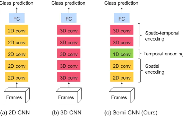
Our proposed framework starts from adopting an existing CNN model as base model to initialize the network architecture. Pre-trained weights for 2D convolution layers are transferred to our semi-CNN to form the bottom layers of our architecture. Temporal convolution layers are then added to form the intermediate structure. Temporal encoding downsamples the depth features while preserving its spatial dimension. Lastly, spatio-temporal encoding layers are added on top before connecting to a fully-connected layer for classification prediction. Figure 1 illustrates the comparison of architecture designs for 2D CNN (Figure 1(a)), 3D CNN (Figure 1(b)), and our semi-CNN model (Figure 1(c)).
Figure 1. Architecture comparison for (a) 2D CNN, (b) 3D CNN and (c) our proposed semi-CNN.
3.1. Base Models
We construct our architecture based on three popular convolutional networks: VGG-16 [20], ResNet [14] and DenseNet [21]. We attempt to preserve the network configurations and model’s depth, while aggregating the layers to perform convolution in the spatial, temporal and spatio-temporal dimensions.
3.1.1. Very Deep Convolutional Networks (VGG)
The architecture of very deep CNN, named VGG, with depth of 16 – 19 layers was introduced by Simonyan and Zisserman [20] for the task of large-scale image classification. The convolution filter size is fixed at 3×3 for all layers to allow deeper implementation while increasing non-linearity functions (by adding a rectification layer after each convolution) to learn complex representations. After the convolution layers, the output is max pooled before connecting to three fully-connected layers of 4096-D. This leads to a high number of learnable parameters, with 138M for VGG-16 layers and 144M for VGG-19 layers.
3.1.2. Residual Networks (ResNets)
output of a previous layer can be mapped and added to the output of the connecting stacked layers. Another benefit of residual learning is that it does not incur additional complexity or parameters to the network, which makes the development of extremely deep network (up to 152 layers) possible, with complexity much lower than VGG nets.
3.1.3. Dense Convolutional Networks (DenseNets)
Another work proposed to build deeper architecture by connecting each convolution layer to all the subsequent layers, forming a densely connected network, DenseNet [21]. Feature maps from previous connected layers were re-used in subsequent layers, hence reducing the number of trainable parameters. Besides, the vanishing gradient problem is also addressed by the skip connections (similar to the shortcut connections in ResNets) between layers, which map the output of a previous layer to the next connecting layer, and allow the gradients from every layer to be accessed during back-propagation. DenseNet has a considerably lower number of parameters when compared with ResNet of the same depth, and yet retains a high training capacity when the model goes deeper. 3.2. Configuration Settings
Our semi-CNN performs spatial convolution first, followed by temporal convolution and finally spatio-temporal convolution. To retain the same network depth as its 2D convolution network, we reduce the number of layers in the spatial convolution blocks and add layers to the temporal and spatio-temporal blocks. When computing the spatial convolution, the output shape of the temporal depth is preserved, and similarly when computing the temporal convolution, the spatial dimension of the output is retained. During spatio-temporal convolution, features are convolved in all three dimensions. For semi-ResNets, residual learning is retained in all the convolutional blocks; while for semi-DenseNets, dense connections between layers in each block are preserved.
Our semi-CNN architecture takes input with dimension 16 × 224 × 224, where 16 denotes the number of consecutive frames, and 224 × 224 denotes the spatial dimension. The input will be passed through spatial convolution blocks and pooling layers to obtain spatial features with an output of size 16 × 14 × 14. Then, the features are convolved with temporal blocks and downsampling to 8 × 14 × 14. At the top layers of the architecture, we perform spatio-temporal convolution and pooling to reduce the feature size to 2 × 3 × 3 or 2 × 4 × 4, before connecting to a global pooling layer to obtain a 1-D representation. The representation will then be passed to fully-connected layers for classification prediction.
3.3. Comparison with 2D and 3D CNN
This section presents a comparison of the layers configuration in 2D, 3D and our semi-CNN, for models VGG, ResNet and DenseNet. The network configuration is simplified and presented in Table 1 for easy reference and comparison.
The notation for the configuration setting for semi-CNN is set as ([ss], tt, [st]), where ss denotes the number of spatial layers with convolutional kernel (1 × x × x), tt denotes the number of temporal encoding layers with kernel size (x × 1 × 1), and st denotes the number of spatio-temporal layers with convolutional kernel size of (x × x × x). The value of convolutional kernel size, x, is set with reference to the configurations in the 2D base model. For instance, the spatial kernel size for semi-VGG-16 is (1 × 3 × 3), while for semi-ResNet-18, the kernel size for the first spatial convolutional block is (1 × 7 × 7). The notation [..] denotes a building block configuration that consists of a stack of convolutional layers. The value shown inside the bracket denotes the number of blocks constructed in the network. Both ResNet and DenseNet models are constructed with building blocks.
Table 1. Configuration comparison for 2D, 3D and semi-CNN architecture, using base model VGG, ResNet and DenseNet.
Model 2D-CNN 3D-CNN Semi-CNN
ResNet-18 BasicBlock [2,2,2,2] BasicBlock [2,2,2,2] BasicBlock ([2,1],[1],[1,1,2]) ResNet-34 BasicBlock
[3,4,6,3]
BasicBlock [3,4,6,3]
BasicBlock ([3,2],[2],[3,3,3]) ResNet-50 Bottleneck
[3,4,6,3]
Bottleneck [3,4,6,3]
Bottleneck ([3,2],[2],[3,3,3]) ResNet-101 Bottleneck
[3,4,23,3]
Bottleneck [3,4,23,3]
Bottleneck ([3,2],[2],[12,11,3]) ResNet-152 Bottleneck
[3,8,36,3]
Bottleneck [3,8,36,3]
Bottleneck ([3,4],[4],[18,18,3]) DenseNet-121 [6,12,24,16] [6,12,24,16] ([6,6],[6],[12,12,16]) DenseNet-169 [6,12,32,32] [6,12,32,32] ([6,6],[6],[16,16,32])
For VGG model, we compare with 2D VGG-16 [20], a 3D convolution network (C3D) [7], and our semi-VGG-16. C3D has 11 layers (8 spatial layer and 3 fully-connected layer), while VGG-16 has 16 layers (13 spatial layers and 3 fully connected layers) in their networks.
For ResNet, we compare with 2D ResNets [14], 3D ResNets [8] and our semi-ResNets. ResNet models are constructed with two types of residual blocks [14] – basic block and bottleneck block. Semi-ResNet is constructed with reference to the building blocks used in the 2D model.
Comparison of DenseNet is the 2D model [21], 3D model (derived from 2D network) and our semi-DenseNet model. Similarly, the network configuration is represented by a stack of building blocks that consists of densely connected layers. Dense connections between layers in each block are preserved in the semi-CNN architecture.
The configurations described in Table 1 are not optimized, but have shown reasonably good performance when validated in the experimental section. A detailed architecture comparison can be found in Table A1 in the Appendix.
4. Experiments
4.1. Implementation Details
We evaluated our framework using the popular action recognition dataset, UCF-101. It contains a total of 13320 video clips, with 101 action classes, and is divided into 3 training-validation splits. In our experiments, we only utilize the split-1 training and validation sets for evaluation. During training, 16 consecutive frames are randomly sampled from each video. Input frames are re-scaled and randomly cropped at multiple scales, before resizing them to the size of 224 × 224. They are also randomly flipped horizontally to allow data augmentation for better training. The input is normalized using the mean and standard deviation of the ImageNet dataset. For validation, the input frames from each validation video are sampled at fixed locations. The frames are rescaled and center cropped, without horizontal flipping.
Our network is trained end-to-end using stochastic gradient descent with learning rate 0.1, momentum 0.9, dampening 0.9, and weight decay of 0.0001. The learning rate is reduced by a factor of 10 when the validation loss value does not decrease for 10 epochs. The network architecture and training is implemented in PyTorch with CUDA, utilizing two GPUs of GeForce RTX2080Ti. Due to memory constraints, we implemented accumulated gradients during training to allow processing of large batch sizes, while retaining the size of the computation graph. We use a mini batch size of 8 (or 4 or 2 depending on the network complexity) and accumulated the gradients for 32 iterations (effective batch size is 256) before back-propagation. The architecture is trained for 50 epochs and we present the validation results for comparison.
4.2. Trainable Parameters
model utilizes transfer learning to initialize our network parameters, we also present the number of pre-trained parameters for each network. The 2D convolution network takes an input of size (48, 224, 224), and its input channel size is 48, while the input dimension for 3D and our semi-convolution is (3, 16, 224, 224), with channel size 3 for each frame’s RGB.
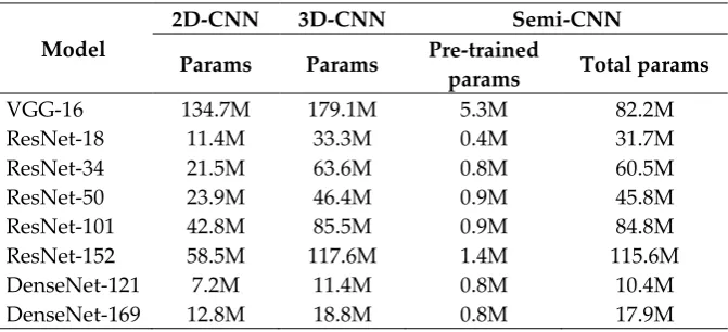
Table 2 describes the number of training parameters for VGG, ResNet and DenseNet models. As can be seen from the table, 3D convolution networks have a much higher number of trainable parameters as compared to their corresponding 2D convolution networks. Our semi-CNN architecture has the lowest number of parameters for the VGG-16 model. As for ResNet and DenseNet models, our network has higher parameters than 2D convolution networks, but lower than 3D convolution networks. The trainable parameters are obtained from the lower layers of the pre-trained network for our spatial convolutions only.
Table 2. Number of training parameters for VGG, ResNet and DenseNet models.
Model
2D-CNN 3D-CNN Semi-CNN
Params Params Pre-trained
params Total params
VGG-16 134.7M 179.1M 5.3M 82.2M
ResNet-18 11.4M 33.3M 0.4M 31.7M
ResNet-34 21.5M 63.6M 0.8M 60.5M
ResNet-50 23.9M 46.4M 0.9M 45.8M
ResNet-101 42.8M 85.5M 0.9M 84.8M
ResNet-152 58.5M 117.6M 1.4M 115.6M
DenseNet-121 7.2M 11.4M 0.8M 10.4M
DenseNet-169 12.8M 18.8M 0.8M 17.9M
4.3. Evaluation on Validation Dataset
This section presents the evaluation results for our architecture and the comparison of its performance with the corresponding 3D-CNN model. Since a previous study [7] has demonstrated that 3D-CNN outperforms 2D-CNN in action recognition tasks, we do not explicitly train 2D-CNN models for our comparison here.
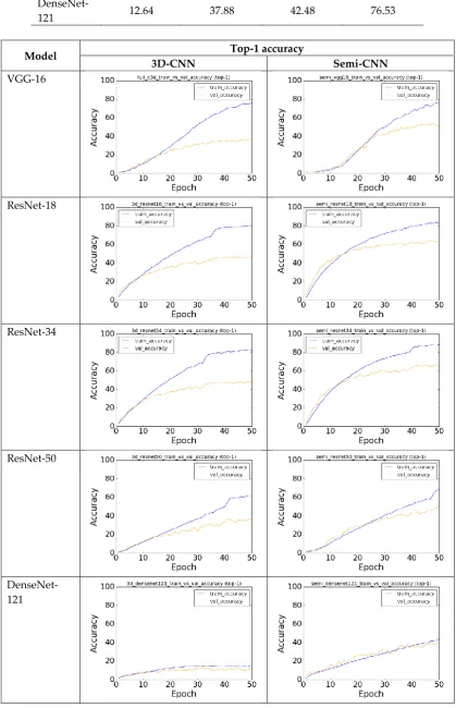
The validation results on UCF-101 Split-1 dataset are presented in Table 3. These results are obtained after training for 50 epochs, which might not have fully converged, but are presented here for comparison and reference. These results show a significant improvement on the prediction accuracy for our semi-CNN when applied on all the different models – VGG, ResNet and DenseNet. For the VGG-16 model, our architecture outperforms C3D [7] by 18% in accuracy. For ResNet models, an average of 16% improvement is achieved, while for the Densenet-121 model, the boost is almost 30%. Deeper networks of ResNet and DenseNet (such as ResNet-101 and DenseNet-169) are not presented here as the validation results deteriorate for both 3D- and semi-CNN architectures, demonstrating that the UCF-101 dataset is too small to be trained for a deep 3D network, as stated in [9, 22]. Figure 2 illustrates the comparison of the training performance for the models listed in Table 3.
Table 3. Comparison of validation results for models VGG, ResNet and DenseNet, with 3D-CNN and semi-CNN architectures.
Model 3D-CNN Semi-CNN
Top-1 acc (%) Top-5 acc (%) Top-1 acc (%) Top-5 acc (%)
VGG-16 36.53 62.70 54.27 81.21
ResNet-18 47.11 73.65 64.92 85.51
ResNet-34 48.19 74.41 66.53 88.58
DenseNet-121 12.64 37.88 42.48 76.53
Model Top-1 accuracy
3D-CNN Semi-CNN
VGG-16
ResNet-18
ResNet-34
ResNet-50
DenseNet-121
In Figure 2, the gap between the training and the validation plots (blue and orange lines) for 3D-CNN models is much bigger as compared to the plots in semi-3D-CNN. This indicates that overfitting occurs when we train a more complex model (or a deeper network) on a relatively small dataset. Our architecture learns faster as can be seen in the steeper slope, which is a result of transfer learning which initializes the parameters in our spatial convolution layers. For deeper networks such as ResNet-50 and DenseNet-121, huge fluctuations can be seen in the validation loss of the 3D architecture, which could mean that the network is overfitting as it could not generalize its training parameters on the validation set. Although fluctuations also occur in our semi-CNN architecture, it is more stable and the validation loss is progressively reduced when trained for more epochs.
This empirical study provides strong support for our semi-CNN architecture in that a fusion of convolution layers outperforms a full 3D convolution network, with additional advantages on: 1) lower number of training parameters, 2) transfer learning from pre-trained models is feasible, and 3) more stable training and faster convergence. Due to our limited computational resources, we only present our validation results on shallower networks on UCF-101 dataset, and we expect that the performance can be generalized to deeper networks when applied on larger datasets.
4.4. Features Visualization and Qualitative Results Comparison
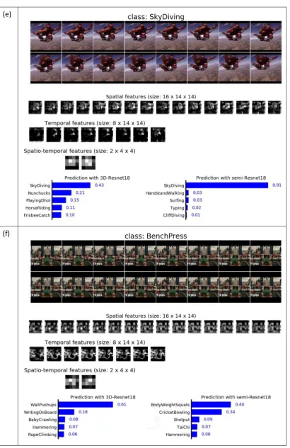
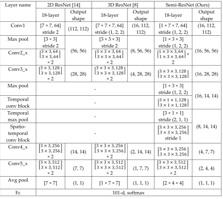
We report the comparisons of qualitative results for 3D- and Semi-ResNet-18 models, as well as illustrations of features for Semi-ResNet-18 in Figure 3. The top two rows of Figure 3 show 16 consecutive frames sampled from the validation video as network input. Subsequent three rows in Figure 3 illustrate examples of features extracted in the spatial, temporal and spatio-temporal space in Semi-ResNet-18 (detailed architecture is presented in Table A1 in the Appendix). Spatial features shown are obtained after the spatial convolution and pooling layers, with output dimension (16 × 14 × 14). After the temporal convolution block and max pooling layer, we obtain temporal features with dimension (8 × 14 × 14). The features are then processed by spatio-temporal blocks, where the output size is further reduced to (2 × 4 × 4). At the bottom row, we illustrate the top-5 prediction scores for both 3D- and Semi-ResNet-18.
(a)
(c)
(e)
(f)
Figure 3. Examples of qualitative results for 3D- and Semi-ResNet-18 for different action classes: (a) Hammer throw, (b) Still rings, (c) Military parade, (d) Wall pushups, (e) Sky diving, and (f) Bench
5. Conclusion
The work in this paper demonstrates the effectiveness of our architecture as compared to existing fusion models and 3D convolution models. We evaluated our architecture on three popular models – VGG, ResNet and DenseNet. Our empirical results show significant improvements over the 3D convolution networks of the three models. In addition, our architecture shows faster convergence with transfer learning and has fewer training parameters which reduces overfitting. The learning properties and the network depth for existing models are preserved. More experiments can be conducted to find the optimal configurations for the spatial, temporal and spatio-temporal convolution layers, as well as the segregation of the layers for each network. Deeper networks can be trained on larger datasets and fine-tuned on UCF-101 to further enhance the prediction accuracy. Author Contributions: Conceptualization, methodology, validation, analysis and draft preparation, M.C; software, resources, funding acquisition and draft review, D.P; supervision, draft review and editing, Y.T; draft review and editing, L.F.
Funding: Please add: “The publication charges for this article have been funded by a grant from the publication
fund of UiT The Arctic University of Norway”.
Conflicts of Interest: The authors declare no conflict of interest.
Appendix A
Table A1. Configuration comparison for 2D ResNet, 3D ResNet and our semi-ResNet, for an 18-layers network.
Layer name 2D ResNet [14] 3D ResNet [8] Semi-ResNet (Ours)
18-layer Output
shape 18-layer
Output
shape 18-layer
Output shape Conv1 [7 × 7, 64]
stride 2 (112, 112)
[7 × 7 × 7, 64] stride (1, 2, 2)
(16, 112, 112)
[1 × 7 × 7, 64] stride (1, 2, 2)
(16, 112, 112) Max pool [3 × 3]
stride 2
(56, 56)
[3 × 3 × 3] stride 2
(8, 56, 56)
[1 × 3 × 3] stride (1, 2, 2)
(16, 56, 56) Conv2_x [3 × 3, 64
3 × 3, 64]
× 2
[3 × 3 × 3, 64 3 × 3 × 3, 64]
× 2
[1 × 3 × 3, 64 1 × 3 × 3, 64] ×
2 Conv3_x [3 × 3, 128
3 × 3, 128]
× 2 (28, 28)
[3 × 3 × 3, 128 3 × 3 × 3, 128]
× 2 (4, 28, 28) [
3 × 3 × 3, 128
3 × 3 × 3, 128] (16, 28, 28)
Max pool
- [1 × 3 × 3]
stride (1, 2, 2)
(16, 14, 14) Temporal
conv block - [
3 × 1 × 1, 128 3 × 1 × 1, 128]
Temporal
max pool -
[3 × 1 × 1] stride (2, 1, 1)
(8, 14, 14) Spatio-
temporal conv block
- [
3 × 3 × 3, 256 3 × 3 × 3, 256]
stride 1 Conv4_x [3 × 3, 256
3 × 3, 256]
× 2 (14, 14)
[3 × 3 × 3, 256 3 × 3 × 3, 256]
× 2 (2, 14, 14)
[3 × 3 × 3, 256
3 × 3 × 3, 256] (4, 7, 7)
Conv5_x [3 × 3, 512
3 × 3, 512]
× 2 (7, 7)
[3 × 3 × 3, 512 3 × 3 × 3, 512]
× 2 (1, 7, 7)
[3 × 3 × 3, 512 3 × 3 × 3, 512]
× 2 (2, 4, 4) Avg pool
[7 × 7] (1, 1) [1 × 7 × 7] (1, 1, 1) [2 × 4 × 4] (1, 1, 1)
Fc 101-d, softmax
1. LeCun, Y., et al., Gradient-based learning applied to document recognition. Proceedings of the IEEE, 1998. 86(11): p. 2278-2324.
2. Soomro, K., A.R. Zamir, and M. Shah, UCF101: A dataset of 101 human actions classes from videos in the wild. arXiv preprint arXiv:1212.0402, 2012.
3. Simonyan, K. and A. Zisserman. Two-stream convolutional networks for action recognition in videos. in Advances in neural information processing systems. 2014.
4. Zhang, B., et al. Real-time action recognition with enhanced motion vector CNNs. in Computer Vision and Pattern Recognition (CVPR), 2016 IEEE Conference on. 2016. IEEE.
5. Gkioxari, G. and J. Malik. Finding action tubes. in Computer Vision and Pattern Recognition (CVPR), 2015 IEEE Conference on. 2015. IEEE.
6. Ji, S., et al., 3D convolutional neural networks for human action recognition. IEEE transactions on pattern analysis and machine intelligence, 2013. 35(1): p. 221-231.
7. Tran, D., et al. Learning spatiotemporal features with 3d convolutional networks. in Computer Vision (ICCV), 2015 IEEE International Conference on. 2015. IEEE.
8. Hara, K., H. Kataoka, and Y. Satoh. Learning spatio-temporal features with 3D residual networks for action recognition. in Proceedings of the ICCV Workshop on Action, Gesture, and Emotion Recognition. 2017.
9. Hara, K., H. Kataoka, and Y. Satoh. Can spatiotemporal 3D CNNs retrace the history of 2D CNNs and ImageNet. in Proceedings of the IEEE Conference on Computer Vision and Pattern Recognition, Salt Lake City, UT, USA. 2018. 10. Feichtenhofer, C., A. Pinz, and A. Zisserman. Convolutional two-stream network fusion for video action
recognition. in Proceedings of the IEEE Conference on Computer Vision and Pattern Recognition. 2016.
11. Tran, D., et al. A closer look at spatiotemporal convolutions for action recognition. in Proceedings of the IEEE conference on Computer Vision and Pattern Recognition. 2018.
12. Yao, T. and X. Li, Yh technologies at activitynet challenge 2018. arXiv preprint arXiv:1807.00686, 2018. 13. Jung, M., J. Hwang, and J. Tani. Multiple spatio-temporal scales neural network for contextual visual recognition
of human actions. in Development and Learning and Epigenetic Robotics (ICDL-Epirob), 2014 Joint IEEE International Conferences on. 2014. IEEE.
14. He, K., et al. Deep residual learning for image recognition. in Proceedings of the IEEE conference on computer vision and pattern recognition. 2016.
15. Varol, G., I. Laptev, and C. Schmid, Long-term temporal convolutions for action recognition. IEEE transactions on pattern analysis and machine intelligence, 2018. 40(6): p. 1510-1517.
16. Tu, Z., et al., Multi-stream CNN: Learning representations based on human-related regions for action recognition. Pattern Recognition, 2018. 79: p. 32-43.
17. Diba, A., V. Sharma, and L. Van Gool. Deep temporal linear encoding networks. in Computer Vision and Pattern Recognition. 2017.
18. Girdhar, R., et al. ActionVLAD: Learning spatio-temporal aggregation for action classification. in CVPR. 2017. 19. Sun, L., et al. Human action recognition using factorized spatio-temporal convolutional networks. in Proceedings of
the IEEE International Conference on Computer Vision. 2015.
20. Simonyan, K. and A. Zisserman, Very deep convolutional networks for large-scale image recognition. arXiv preprint arXiv:1409.1556, 2014.
21. Huang, G., et al. Densely connected convolutional networks. in Proceedings of the IEEE conference on computer vision and pattern recognition. 2017.