Tuning a Semantic Relatedness Algorithm using a
Multiscale Approach
Jos´e Paulo Leal1and Teresa Costa2
1 CRACS & INESC-Porto LA, Faculty of Sciences, University of Porto
Porto, Portugal [email protected]
2
CRACS & INESC-Porto LA, Faculty of Sciences, University of Porto Porto, Portugal
Abstract. The research presented in this paper builds on previous work that lead to the definition of a family of semantic relatedness algorithms. These algorithms depend on a semantic graph and on a set of weights assigned to each type of arcs in the graph. The current objective of this research is to automatically tune the weights for a given graph in order to increase the proximity quality. The quality of a se-mantic relatedness method is usually measured against a benchmark data set. The results produced by a method are compared with those on the benchmark using a nonparametric measure of statistical dependence, such as the Spearman’s rank correlation coefficient. The presented methodology works the other way round and uses this correlation coefficient to tune the proximity weights. The tuning process is controlled by a genetic algorithm using the Spearman’s rank correlation coeffi-cient as fitness function. This algorithm has its own set of parameters which also need to be tuned. Bootstrapping is a statistical method for generating samples that is used in this methodology to enable a large number of repetitions of a genetic algo-rithm, exploring the results of alternative parameter settings. This approach raises several technical challenges due to its computational complexity. This paper pro-vides details on techniques used to speedup the process. The proposed approach was validated with the WordNet 2.1 and the WordSim-353 data set. Several ranges of parameter values were tested and the obtained results are better than the state of the art methods for computing semantic relatedness using the WordNet 2.1, with the advantage of not requiring any domain knowledge of the semantic graph.
Keywords:Semantic similarity, Linked data, Genetic algorithms, Bootstrapping, WordNet
1.
Introduction
This paper is an extended version of paper presented at the Symposium on Languages, Applications and Technologies [17] and presents ongoing work aiming the development of a new methodology to determine the semantic relatedness between a pair of concepts. This methodology is knowledge based, it is applied to a semantic graph and does not require any knowledge about the graph’s domain. It uses a family of semantic related-ness algorithms based on the notion of proximity [16]. An algorithm from this family is parametrized by a semantic graph, where the resources are the graph nodes and the prop-erties the arcs. Each type of arc has a specific weight value. Tuning these weights in order to improve the quality of the semantic relatedness is the current objective of this research. There are other methods based on semantic graphs available in the literature [1, 21, 31] that measure the quality of their algorithms using as benchmark a standard data set [11]. This data set has the reference similarity of concept pairs that is the average similarity assigned by a group of persons. The relatedness computed with an algorithm is compared against those of the benchmark using a nonparametric measure of statistical dependence, such as the Spearman’s rank correlation, and its quality is as high as the value of the correlation.
A measure of quality is essential for using a genetic algorithm in a tuning process. In this tuning approach, an assignment of values to weights is encoded as a set of genes of a chromosome. New chromosomes are obtained by crossover and mutation of chromo-somes from the previous generation where the best are selected using a fitness function. The fitness function receives as input a weight assignment and returns the Spearman’s rank order correlation for a subset of benchmark data.
The genetic algorithm has in turn its own set of parameters that need to be tuned. Bootstrapping is a statistical procedure that produces a larger number of samples that are used to explore the most promising settings of the genetic algorithm. The best setting is finally used to run the genetic algorithm a larger number of times with the complete data set.
The tuning approach was validated with the semantic graph of WordNet 2.1 [10], us-ing as benchmark the WordSimilarity-353 [11] data set. The obtained results are better than the best result available in the literature for the same knowledge source and bench-mark [31].
Due to its computational complexity, the tuning approach raises several technical chal-lenges. Firstly, the semantic algorithms must collect a large number of paths connecting each pair of labels in the graph. Secondly, in order to compute the Spearman’s rank order correlation, the semantic relatedness algorithm must be executed with several hundreds of pairs of concept labels. Thirdly, the genetic algorithm must compute a correlation for each chromosome (a set of weight assignments) in the genetic pool for hundreds of generations. And finally, the evolution process of the genetic algorithm has to be repeated hundreds of times as part of the bootstrapping method. This paper also presents approaches used to speedup the tuning process.
2.
Related Work
Semantic measures, such as semantic relatedness, are widely used to estimate the strength of a semantic relationship between elements. The information needed to estimate those measures can be extracted from two different source types.
Sources of the first type are unstructured or semi-structured texts. These texts have ev-idences of semantic relationships among their content. In order to estimate the strength of a semantic relationship it is possible to use simple assumptions regarding the distribution of words. Sources of the other type are structured and explicit knowledge representa-tions. Semantic measures based on this source type rely on semantic graph processing techniques. The approaches of computing semantic measures are based on the type of the source: the distributional methods, the knowledge-based methods and the hybrid methods. The distributional approaches use unstructured texts analysis. They compare words, sentences or documents and their occurrence. These approaches rely on thedistributional hypothesis[14] which states that words occurring in similar contexts tend to be seman-tically close. This means that words surrounded by the same words (similar context) are likely to be semantically similar. There are several methods following this approach, such as the spatial/geometric methods, the set-based methods and the probabilistic methods.
The spacial/geometric methods assume a semantic space where a word, for instance, is a point in a multi-dimensional space that represents the diversity of the vocabulary used. Two words are compared regarding their location in the multi-dimensional space. An example of this approach is found in Ganesan [12] work.
The set-based methods compare words regarding their context, considering which are common and which are different, using classical set-based measures such as the Dice index or the Jaccard coefficient. The work of Bollegala [5] and Terra & Clarke [32] are examples of this type of methods.
The probabilistic methods express the semantic relatedness of words in terms of prob-ability of co-occurrence. They consider both the contexts in which the compared pairs of words appear and the contexts in which the two words co-occur. These evidences are used to estimate the semantic relatedness. This type of methods were used by Dagan [7] in his work.
Distributional approaches do not require prior knowledge of the meaning and usage of words, but they have some limitations; they are highly dependent of the corpus used and words to compare must occur at least few times. They also require word disambiguation process prior to comparison.
The knowledge-based approaches rely on structured data, such as semantic graphs. They consider the structural properties of the graph and elements are compared by study-ing their interconnections and the semantic of those relationships. Different methods have been defined to compare elements in a single knowledge base and also in multiple knowl-edge bases, such as structural methods, feature-based methods and Shannon’s Information Theory methods.
rela-tionships connecting the elements. Examples of this approach are the work of Rada [26], Resnik [28] and Li [18, 19].
The feature-based methods estimate the semantic relatedness considering specific properties of the elements during the process. These methods need a function to char-acterizefeaturesof the elements that will be compared. The semantic relatedness is ob-tained by evaluating the number of features they share. Bodenreider [4], Stojanovic [30] and Ranwez [27] followed these methods.
There are also methods based on the Shannon’s Information Theory. In these methods, the elements are compared using the amount of information they share and the amount of information they have distinct. Lin [20] and Pirr´o [25, 23, 24] developed their approaches based on this type of methods.
With knowledge-base approaches is possible to compare every pair of elements rep-resented in the graph and also control which properties should be considered in the eval-uation. These methods are easier to implement than the distributional methods and have a lower complexity. However they require a knowledge representation describing the ele-ments.
There are also hybrid approaches that mix knowledge-base and distributional ap-proaches. These methods take advantage of both texts and knowledge representations to estimate the semantic relatedness. Examples of these methods are given by Resnik [28], Banerjee & Pedersen [2, 3] and Patwardhan [22].
The methodology presented in this paper follows a knowledge-based relying in struc-tural methods as detailed on the next section.
3.
Previous Work
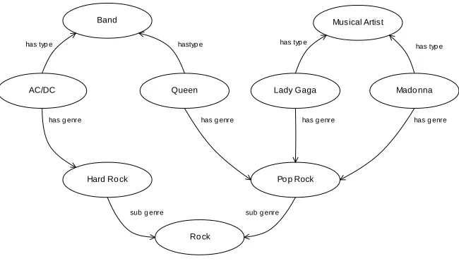
Concepts in semantic graphs are represented by nodes. Take for instance the music do-main. Singers, bands, music genres, instruments or virtually any concept related to music is represented as nodes in a knowledge representation. These nodes are related by proper-ties, such ashas genreconnecting singers to genres, and thus form a graph.
The semantic relatedness measure in development in this research uses a semantic graph to compute the relatedness between nodes. Actually, the goal is the relatedness between concepts, but concept nodes of semantic graphs typically have a label — a string representation or stringification — that can be seen as a term.
At first sight relatedness may seem to be the inverse of the distance between nodes. Two nodes far apart are unrelated and every node is totally (infinitely) related to itself. Interpreting relatedness as a function of distance has an obvious advantage: computing distances between nodes in a graph is a well studied problem with several known algo-rithms. After assigning a weight to each arc one can compute the distance as the minimum length of all the paths connecting the two nodes.
On a closer inspection this interpretation of relatedness as the inverse of distance reveals some problems. Consider the graph in Figure 1. Depending on the weight assigned to the arcs formed by the propertieshas typeandhas genre, the distances between Lady Gaga, Madonna and Queen are the same. If thehas genrehas less weight than
thanhas genrethen Queen is more related to AC/DC than to Lady Gaga or Madonna simply because they are both bands, which also should not be the case.
Band Musical Artist
Lady Gaga Mado nna
Queen
Po p Rock
has g enre hastyp e has typ e
has typ e
AC/DC
Hard Ro ck
has typ e
has g enre has g enre
has g enre
Ro ck
sub g enre sub g enre
Fig. 1.RDF graph for concepts in music domain
In the proposed semantic relatedness measure, we considerproximityrather than dis-tance as a measure of relatedness among nodes. By definition3, proximity is closeness; the state of being near as in space, time, or relationship. Rather than focusing solely on min-imum path length, proximity balances also the number of existing paths between nodes. As an example consider the proximity between two persons. More than resulting from a single common interest, however strong, it results from a collection of common interests. With this notion of proximity, Lady Gaga and Madonna are more related to each other than with Queen since they have two different paths connecting each other, one through
Musical Artistand anotherPop Rock. By the same token the band Queen is more related to them than to the band AC/DC.
Our insight is that an algorithm to compute proximity must take into account all the relevant paths connecting two nodes and their weights. However, paths are made of several arcs, and the weight of an arc type should contribute less to proximity as it is further away in the path. In fact, there must be a limit in number of arcs in a path, as semantic graphs are usually connected graphs.
In this methodology, the estimation of a proximity value depends on exploring a graph. In a semantic graph a node can be linked to other node by several typed arcs. Although semantic graphs are usually characterized as directed multigraphs4, for the purpose of this semantic measure the semantic graph can be interpreted as an undirected graph since, in
3
https://en.wiktionary.org/wiki/proximity
4
general, it is possible to define an inverse relationship for each arc type in the graph. A domain graph can be defined asG= (V, E, T, W)whereV is the set of nodes (concepts),
Eis the set of edges connecting the nodes,T is a set of edges types andW is a mapping of edges types to weight values. Each edge inEis a triplet(u, v, t)whereu, v ∈V and
t∈T.
The setW defines a mapping w: T 7→ N+ and the upper bound of weights for all
types is
Ω(G)≡maxti∈Tw(ti)
In order to retrieve the proximity between two concepts it is necessary to walk through the graph and build a set of distinct paths that connect them. A pathpof sizen∈N+is a
sequence of unrepeated nodes in{u0. . . un|(∀i, j, n)((0≤i≤j≤n)∧(ui6=uj))}that
are linked by typed arcs, that must have at least one edge and cannot have loops; paths are denoted as follows.
p=u0
t1 −→u1
t2
−→u2. . . un−1
tn
−→un
The weight of a pathpis the sum of the weights of each edge and the weight of an edge depends on its type,ω(p) =w(t1) +w(t2) +. . .+w(tn). The set of all paths of sizen that connect two concepts is defined as follows.
Pu,vn ={u0
t1
−→u1. . . un−1
tn
−→un:u=uo∧v=un∧ ∀i,j,n0≤i≤j≤n∧ui 6=uj}
The weight ofPn
u,vis the sum of all sub paths that connectsuandv. The algorithm used
to calculate proximity is based on this definition but also considers the path length. The shorter the path the higher is its contribution to the proximity.
The proximity functionris defined by the following formula, where∆is the graph maximum degree.
r(u, v) =
1 ←u=v
1
Ω(G)
∞
P
n=1 1 2nn∆(G)n
P
p∈Pn u,v
ω(p) ←u6=v (1)
Given a graph with a set of nodesV
r:V ×V 7→[0,1]
The proximity functionr takes two nodes and returns a “percentage” of proximity be-tween then. This means that the proximity of related nodes must be close to1 and the proximity of unrelated nodes must be close to0.
The main issue with this definition of proximity5is how to determine the weights of transitions. The first attempt was to define these weights using domain knowledge. For instance, when comparing musical performers one may consider that being associated with a band or with another artist is more important than their musical genre, and that genre is more important than their stylistics influences and even more important than instruments they play.
However this na¨ıve approach to weight setting raises several problems. Firstly, this kind of “informed opinion” frequently has no evidence to support it, and sometimes is
5
plainly wrong. How sure can one be that stylistics influences should weight more than the genre in musical proximity? Even if it is true sometimes, how can one be sure it is true in most cases? Secondly, this approach is difficult to apply to a large ontology encompassing a broad range of domains. Is a specialist required for every domain? How should an ontology be structured in domains? What domain should be considered for concepts that fall in multiple domains? To be of practical use, the weights of a proximity based semantic relatedness algorithm must be automatically tuned.
4.
Multiscale Weight Tuning
This section describes an approach for tuning weights in a family of semantic relatedness algorithms. The proposed tuning approach operates at different scales. Although each scale has its own distinctive features, there are self-similar patterns common to all scales. In this tuning approach, the common pattern is the concept of function, with input and output values, and a set of parameters that can be tuned. At the lowest scale this function computes the quality of a semantic relatedness algorithm. It takes as input the parameters of semantic relatedness algorithm and produces a numeric value, a semantic relatedness measure. This function takes as parameters a semantic graph and a set of weights that must be tuned.
Zooming out to the next scale, there is a genetic algorithm. A genetic algorithm can be seen as a function taking as input a fitness function and producing a result. It has also its own set of parameters that need to be tuned such as the number of generations and the mutation rate. In this case the fitness function takes as input a set of weights and computes its quality. Hence, each application of a genetic algorithm (seen as a function) aggregates thousands of applications of functions from the previous scale.
Continuing to zoom out to the next and final scale there is a statistical method, the bootstrapping method. This method measures the accuracy of the results obtained by the genetic algorithm with different parameter sets. It can also be seen as a function taking as input genetic algorithms, the candidates for producing a weight tuning, and producing an estimate of which is the best. Again, each application of the bootstrapping method (seen as a function) aggregates thousands of applications of the functions from the previous scale – the genetic algorithm – since each candidate configuration set is repeated hundreds of times. The following subsections detail each of these “scales” and describes the function that is used as input for its upper scale, identifying its parameters.
4.1. Quality Measure
of a set weight attributions. Each of the following subsections details these steps to define the quality of a semantic related measure.
Negative weight values To cope with the negative weight values a few adjustments must
be made to the original definition. First of all the upper boundΩ(G), must be redefined using the absolute value of all weights.
Ω(G)≡maxti∈T|w(ti)|
The purpose of this upper bound is to constrain the semantic measure to a known in-terval (originally[0,1]). Since the definition in (1) relies on an infinite series one must ensure that it converges. Given that if u 6= v then Pn
p∈Pu,vw(p) ≤ Ω(G)n∆(G) n
hence r(u, v) ≤ P∞
n=11/2
n = 1. For non-negative weight values it is trivial that r(a, b) ≥ 0. With negative weights and considering the redefinition of Ω(G) results thatPn
p∈Pu,vw(p) ≥ −
Pn
p∈Pu,v|w(p)| ≥ −Ω(G)n∆(G)
n hence the lower bound is
r(u, v) ≥ −P∞
n=11/2
n =−1. Thus, with negative weights and the new definition of Ω(G)the proximity functionris now defined as
r:V ×V 7→[−1,1]
It would be trivial to adjust the definition of functionrto maintain its original codomain. However, since the codomain itself is not important, as far as it has known boundaries, it was decided to preserve the original definition given in (1).
Factoring out weights The first step is to express proximity in terms of weights of
arc types. Consider the set of all arc typesT with]T = mand the weights of its ele-mentsw(t),∀t ∈ T. The second branch of (1) can thus be rewritten as follows, where ci(a, b), i∈ {1..m}are the coefficients of each arc type.
r(a, b) =α
∞
X
n1
β X
Pj∈P X
t∈Pj
w(t) =
m
X
i=1
ci(a, b)·w(ti)
It should be noted that the weights of transitions types are independent of arguments of r but the coefficients that are factored out depend of these arguments. By defining a standard order on the elements of T both the weights of transitions and their coef-ficients are representable as vectors, respectively (w(t1), w(t2), . . . , w(tk)) = w and
(c1(a, b), c2(a, b), . . . , cm(a, b)) = c(a, b). This way the previous definition of r may
take as parameter the weight vector as follows
rw(a, b) =c(a, b)·w (2)
Quality as function of weights The usual method for estimating the quality of a semantic relatedness function is to compare it with a benchmark data set. The benchmark data set contains pairs of words and their relatedness.
Rather than the simple correlation between the two data series, the Spearman’s rank order sorts those data series and correlates their rank.
Consider a benchmark data set with the pairs of words(ai, bi)for1 ≤i ≤k, with a proximity xi. Given the relatedness functionrw : S ×S 7→ < let us define yi =
rw(ai, bi). In order to use the Spearman’s rank order coefficient bothxiandyimust be
converted to the ranksx0i andy0i. The quality of the function is given by the Spearman’s rank orderρdefined as
ρ=
P
i
(x0i−x0)(y0
i−y0)
r P
i
(x0i−x0)2P
i
(yi0−y0)2
The Spearman’s rank order coefficient is thus defined in terms ofxiandyi, wherexi
are constants from the benchmark data set. To use this coefficient as the fitness function it must be expressed as a function ofw. Considering thaty= (rw(ai, bi), . . . , rw(an, bn)) theny=CwwhereCandware the following matrices.
C=
ca1b1
t1 . . . c
a1b1
tm . . . . . .
canbn
t1 . . . c
anbn tm w=
w(t1)
. . . . . .
w(tm)
MatrixC is an×mmatrix where each line contains the coefficients for a pair of concepts and each column contains coefficients of a single edge (transition) type. Vector wis am×1matrix with the weights assigned to each edge type. The product of these matrices is the proximity measure of a set of concept pairs.
Consideringρ(x,y)as the Spearman’s rank order ofxandy, the quality function
q:<n7→ <using the benchmark data setxcan be defined as
qx(w) =ρ(x, Cw) (3)
The next step in this tuning methodology is to determine aw that maximizes this quality function.
4.2. Genetic Algorithm
Genetic algorithms are a family of computational models that mimic the process of natural selection in the evolution of the species. These algorithms use the concepts ofvariation, differential reproduction andheredity to guide the co-evolution of a set of problem so-lutions. This type of algorithm is frequently used to improve solutions of optimization problems [33].
next generation (differential reproduction). At last, the representation of solutions as in-dividuals must allow their recombination with other solutions (heredity) so that favorable traits are preferred over unfavorable ones as the population of solutions evolves.
In this weight tuning approach, theindividualis a vector of weight values. Consider a sequence of weightsw(t1), w(t2). . . w(tk)(the genes) taking values in natural numbers up to a certain limit in a standard order of arc types. Two possible solutions are the vectors
v = (v1, v2, .., vk)andt = (t1, t2, . . . , tn). They are easy to recombine by crossover,
taking “genes” from both “parents” (e.g.u= (v1, t2, . . . tn−1, vk)).
This representation contrasts with the binary representations typically used in genetic algorithms [9]. However it is closer to the domain and it can be processed more efficiently with large number of weights.
Genetic algorithms introduce variance also bymutation. There is a number of muta-tion operators, such as swap, scramble, insermuta-tion, that can be used on binary representa-tions [9]. However, the approach taken to represent individuals in this methodology makes these operators inadequate. Since weights are independent from each other, swapping val-ues among them is as likely to improve the solution as selecting a new random value. Hence, the genetic algorithm created for tuning weights has a single kind of mutation: randomly selecting a new value for a given “gene”.
The fitness function plays a decisive role in selecting the new generation of individu-als, created by crossover and mutation of their parents. In this case individuals are a vector of weight valuesw, hence the fitness function is in fact the quality function defined by equation (3).
4.3. Bootstrapping
The genetic algorithm itself has a number of parameters that must be tuned. Generic parameters of a genetic algorithm include the number of generations and the mutation rate. In this particular case the range of values that may be assigned to weights must also be considered.
Several approaches to tuning parameters of genetic algorithms have been proposed and compared [29]. Although with different approaches, these methods highlight the ad-vantage of using automated parameter tuning over tuning based on expert “informed opin-ions”. In many cases the best solution contradicts the expert best intuitions.
The proposed approach relies on a single benchmark data set to compare alternative weight attributions. To repeat a large number of experiments using the genetic algorithm to co-evolve a set solutions one needs a larger number test samples. Bootstrapping [8] is a statistical method for assigning measures of accuracy to data samples using a simple technique known asresamplingthat solves this issue.
Resampling is applied to the original data set to build a collection of sample data sets. Each sample data set has the same size as the original data set and is built from the same elements. If the original data set has sizenthennelements from that set are randomly chosen to create the sample set. When an element is selected it is not removed from the original data set. Hence, a particular element may occur repeatedly on the sample data set while other may not occur at all.
quartile. In the end, these statistics are compared to select the most effective combination. Since the objective is to select the set of parameters that may lead to the highest quality, the third quartile is specially relevant since it is a lower bound of the largest solutions.
In this tuning approach, each combination corresponds to a particular setting of the genetic algorithm. Candidate settings include values for parameters such as the number of generations or the mutation rate. Another important parameter that is specific to this approach is the range of values that are used as possible values for weights. As these val-ues have to be enumerated, this procedure considers only integer valval-ues bellow a certain threshold.
As the result of the bootstrapping method a particular setting of the genetic algorithm’s parameters is selected. The final stage is to run the genetic algorithm with these settings, using the full benchmark data set in the fitness function. The selected genetic algorithm is repeated an even larger number of times, typically 1000, and the best result is selected as weights for the relatedness algorithm.
5.
Implementation
The approach presented for parameter tuning has a high computational complexity. At its core it has to find all paths connecting two concepts to compute a single proximity. To test the quality of a vector of weights, the proximity has to be computed for each pair of concepts in a benchmark data set. Bootstrapping repeats 200 times the genetic algorithm for each setting, and this process is repeated for a large number of settings.
The proximity measure takes two strings as labels and builds a set with all the paths that connect both terms. There is a label stemming process that explores the meaning of related words or expressions. For instance, when one of the compared term is “book”, then nodes having as labels “bookish” and “book shop” may also be explored. The stemming process is a special kind of transition and may improve the quality of the relatedness measure, but also increases the computational complexity of the tuning process.
Figure 2 provides an overview of the proposed semantic relatedness methodology. The process begins with the graph pre-processing. This action is not mandatory but is crucial to improve the efficiency, as detailed in the subsection 5.1.
The process itself is parametrized by a data set and begins with the bootstrap proce-dure that tests a user defined set parameters - mutation rate, number of generations and weight range - for different values. Each specific set of parameters is tested 200 times and is summarized by statistic measures that are decisive to choose the best set of parameters. Each set of parameters is tested by the genetic algorithm. To generate a weight as-signment, the genetic algorithm runs the number of generations defined by the parame-ters. This weight assignment is used by the proximity algorithm that returns the weight’s quality. In the end, the best quality is selected.
A weight assignment is tuned by using the proximity algorithm. The semantic re-latedness of each pair of words of the data set is tested using the proximity algorithm and its value is compared against the benchmark value using the Spearman’s correlation, returning the quality of the given assignment.
Graph Proximity
Genetic
opt # generations
Control Bootstrap
opt x200
preProcessing()
tuneGenetic (params)
tuneProximity (weights)
proximity(pair)
value
opt dataset
Spearman()
quality
processing(dataset)
getBestSetting()
bestParameters
tune(bestParameters, dataset)
getBestQuality()
bestQuality
loop loop
loop
opt # generations
tuneProximity (weights)
proximity(pair)
value
opt dataset
Spearman()
quality
getBestQuality()
loop loop
quality
opt all settings
loop
opt x1000
loop
Fig. 2.Methodology diagram
The strategy used for improving the efficiency of the methodology has three main components: graph pre-processing, described in the subsection 5.1; factorization of the proximity algorithm and concurrent evaluation of the bootstrapping method, described in the subsection 5.2. The remainder of this section details each of these components.
5.1. Graph Pre-processing
response. Paths are built from data collected by the exploratory methods using SPARQL queries.
The initial step is to retrieve the set of nodes linked to each term of the process. Since this methodology estimates the semantic proximity between a pair of terms, this method is executed twice. For each node retrieved during all the process, the second exploratory method fetches the list of nodes that are connected to it. Whenever is possible to build a path between both terms using the expanded nodes and its transitions, that path is con-sidered to measure the proximity. This traverse ends when there are no more nodes to explore or when the path size limit is reached.
This SPARQL approach raises a number of issues. Firstly, the endpoint or network may be under maintenance or with performance problems. Secondly, some endpoints have configuration problems and do not support queries with some operators, such asUNION. And thirdly, the SPARQL queries can have performance issues, mainly when using oper-ators such asDISTINCT, and having a large amount of queries per proximity search can cause a huge impact at the execution time.
In order to avoid those issues, this semantic relatedness methodology implements searches in local data. Knowledge bases often provide dumps of their data. Local data are pprocessed semantic graphs that are stored in the local file system with data re-trieved from those dumps. Graph pre-processing begins with parsing the RDF data. RDF data can be retrieved in several formats, such as Turtle, RDF/XML or N-Triples. To sim-plify this process, all RDF data is converted to N-Triples, since this is the simplest RDF serialization.
This process takes some time to execute but it is only necessary to execute once. Also, the most used data is cached in memory which has a significant impact on performance.
The computation of the proximity of a single pair of concepts using the WordNet 2.1 SPARQL endpoint6 takes about 20 minutes. With the pre-processed graph7 that is executed once and takes 30 minutes, the same computation takes about 6 seconds.
5.2. Other Optimizations
Traversing the graph searching for paths connecting two labels is the most frequently executed part of this semantic relatedness methodology. Nevertheless, this procedure is almost the same for each pair of concepts, varying only on the weights that are used for each arc type. This computation is repeated many times since the exact same pair of concepts is used each time that the genetic algorithm is run.
The solution found was to alter the proximity algorithm to compute the set of coef-ficients that are multiplied to each weight. These coefcoef-ficients are organized in a vector, using the same order of the weight vector used in the genetic algorithm. Thus, computing the proximity of a pair of concepts given a different weight vector is just the inner product of the weight vector and the coefficient vector, as shown in (2).
With this modification a single run of the genetic algorithm with 200 generations takes less than 1 minute and computing the coefficients for all the pairs takes about 30 minutes. The final optimization was concurrent evaluation of the bootstrapping method. Each of the settings can be processed independently, hence they could be assigned to a different
6wordnet.rkbexplorer.com/sparql/ 7
processor of a multi-core machine7. Each run of the bootstrapping method takes about 200 minutes. It run 120 configurations that sequentially would have taken more than 16.5 days in about 2 days.
6.
Validation
The validation of the proposed tuning approach consisted of tuning the weights of the relatedness algorithm for WordNet 2.1.
The WordNet8 [10] is widely used in most of the mentioned knowledge-based ap-proaches [6, 15, 1, 21, 31]. It is a large lexical knowledge base for English words. It groups nouns, verbs, adjectives and adverbs intosynsets(set of cognitive synonyms) that express distinct concepts. Synsets are interlinked by lexical and conceptual-semantic relation-ships. This knowledge-base is well-known but lacks some specialized vocabularies and named entites, such as Diego Maradona or Freddie Mercury. WordNet 2.1 is a compar-atively small knowledge base with 26 different types of properties that interlink 464.795 nodes and thus it is ideal for the inital tests of a tuning methodology.
This tuning process used as benchmark the WordSimilarity-353 data set [11]. It has 353 pairs of concepts with the mean of the relatedness values given by humans. Since WordNet 2.1 does not have all the words listed in this data set, the pairs with missing elements were removed, creating a new data set with the non-missing pairs. In total 7 pairs were removed.
The tuning was performed in two rounds. In the first round a large number of settings was explored to determine which were the most relevant. A second round was then per-formed to explore a wider range of values on those parameters that have more impact on performance.
5 10 15 20
0.00
0.10
0.20
0.30
negative 3rd quartile negative mean positive 3rd quartil positive mean
Amount of weight values
Spear
man's r
ank order
mixed 3rd quartile mixed mean positive 3rd quartil positive mean
Fig. 3.Graph of weights distribution
8
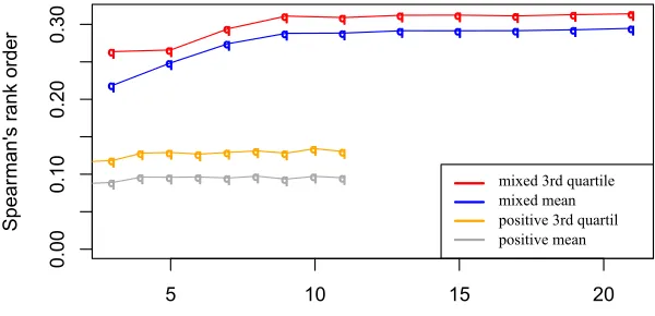
In the first round the bootstrapping process tested three parameters: weight values, mutation rate, and number of generations. The weight values were divided in positive and mixed (positive and negative) values; the positive values ranged in[0, n]withn ∈
N+ andn ≤ 10. The mixed values ranged in [−n, n]for the same values of n. The
mutation rate took values in the set{0.3,0.4,0.5}values and the number of generations in{100,200}. Permutating these values, 120 different sets of parameters were tested. Each set of parameters was executed 200 times in the bootstrapping process. The results of those tests can be seen in the following graphs. These graphs show the statistics of the correlation as function of a single variable: number of weight values, mutation rate and number of generations.
Figure 3 shows how the correlation varies with different ranges of weight values. The correlation obtained when there are only positive values in the weight set is much lower than when positive and negative weights are used. The positive values also appear to reach a maximum value. However, the sets with positive and negative values do not show that stabilization, suggesting the need for more tests with a larger range of values. Third quartile and mean were used in order to verify if the variations were consistent.
M3=0.3 M4=0.4 M5=0.5
−0.1
0.0
0.1
0.2
0.3
0.4
Mutation Values
Spear
man's r
ank order
G1=100 G2=200
−0.1
0.0
0.1
0.2
0.3
0.4
Generation Values
Spear
man's r
ank order
Fig. 4.Distribution of different mutation rates (left) and number of generations (right)
The graph on the left of Figure 4 shows the impact of changing the mutation rate. Despite the large overall variation, the mean and third quartile values are similar, showing that variations in this parameter have a small impact on the tuning process. Still, the variation of the maximums indicate the relevance of also testing lower mutation rates in the future.
After the first round, changes in range of weight values appear to have a higher impact in the correlation values, specially if they allow negative values, increasing the correlation as the range size increases. New tests were conducted to investigate for how long the correlation continues to increase, if it converges to an asymptote, or if the correlation degrades after a certain threshold.
A new round of tests was made to investigate these hypothesis. This time only pos-itive and negative values were used, with fixed values of mutation rate and number of generations. These new configurations uses ranges from[−10×n,10×n]withn∈N+
andn≤10. The mutation rate value was fixed at0.4and the number of generations was fixed at200. The results are displayed in Figure 5. The values obtained by increasing the range of values show a maximum value at the range [-20,20]. Ranges with higher values seem to never exceed the Spearman’s rank order obtained at that point, indicating that performance degrades after this threshold.
0 50 100 150 200
0.22
0.26
0.30
negative 3rd quartile negative mean
Amount of weight values
Spear
man's r
ank order
mixed 3rd quartile mixed mean
Fig. 5.Graph of weights distribution
Using the best configuration obtained by the bootstrap process the genetic algorithm was executed 1000 times aiming to obtain the best correlation value and the related con-figuration.
The best Spearman’s rank order value obtained was 0.409 and the corresponding weight set is listed in the Table 1. The arcs with the prefixwncorrespond to the WordNet 2.1 URI9and the prefixrdfsto the RDF Schema URI10. The arc type:stemmingis the custom arc created in the stemming process.
Table 2 compares the results obtained by our semantic measure with weights tuned by the proposed methodology with other similar semantic measures described in the litera-ture, that use also the WordNet 2.1 as semantic graph and that validate their results using WordSim-353.
9
http://www.w3.org/2006/03/wn/wn20/schema/
10
Table 1.Weight values obtained after tuning process
Edge type Weight Edge type Weight
:stemming 1 wn:classifiedByUsage 18
wn:memberMeronymOf -2 wn:tagCount 1
wn:participleOf -6 wn:sameVerbGroupAs -8 wn:antonymOf -5 wn:derivationallyRelated 0 wn:classifiedByTopic 19 wn:attribute -15
wn:partMeronymOf 19 wn:synsetId 18
wn:word 12 wn:seeAlso 6
wn:gloss 19 rdfs:type -2
wn:similarTo -19 entails -1
wn:containsWordSense 4 wn:classifiedByRegion -9
wn:causes -17 wn:adverbPertainsTo 12
wn:frame 7 wn:hyponymOf 9
wn:adjectivePertainsTo 3 wn:substanceMeronymOf 18
Table 2.Previous work with WordNet and WordSim-353
Method Spearman’s rank order
Jarmasz (2003) 0.33 - 0.35
Strube and Ponzetto (2006) 0.36
Proposed methodology 0.41
7.
Conclusion
The major contribution of the research presented in this paper is an approach for tun-ing a relatedness algorithm to a particular semantic graph, without requirtun-ing any domain knowledge on the graph itself. The results obtained with this approach for WordNet 2.1 are better than the state of the art for the same graph. A number of solutions to speedup graph processing and the evaluation of fitness functions are also relevant contributions.
The proposed approach performs a multiscale parameter tuning of a graph based se-mantic relatedness algorithm. The main feature of the base algorithm is the fact that it considers all paths that connect two labels and computes the contribution of each path as a function of its length and of the arc (properties) types. The main issue with this algo-rithm is the selection of parameters (weight values for each arc type) that maximize the quality of the relatedness algorithm.
The proposed approach for tuning the parameters of the semantic relatedness algo-rithm was validated with Wordnet 2.1. The tuning procedure was actually executed twice. In the first run several parameters of the genetic algorithm were tested to conclude that the range of weight values is the decisive parameter, in particular if it is allowed to contain negative values. The variation of some of the parameters, such as mutation rate and num-ber of generations, had no impact on the quality. Based on these findings a second run of the tuning procedure explored a wider range of values. It showed that quality improves with the width of range values but also that a small degradation occurs after a certain threshold. The genetic algorithm was finally repeated a large number of times with the settings selected by this approach and the maximum Spearman’s correlation obtained is significantly higher than the best result reported on the literature for the same graph.
The Wordnet 2.1 graph used for the evaluation is comparatively small. It has just 26 different types of properties and 464.795 nodes. The next step is to investigate how this approach works with Wordnet 3.0 and with even larger graphs, such as the DBPedia or Freebase. Apart from the challenges of dealing with such large graphs, it will be interest-ing to compare the semantic relatedness potential of different graphs and try to combine them to improve the accuracy of the semantic relatedness algorithm.
Acknowledgments.This work is financed by the ERDF European Regional Development Fund through the COMPETE Programme (operational programme for competitiveness) and by National Funds through the FCT — Fundac¸˜ao para a Ciˆencia e a Tecnologia (Portuguese Foundation for Science and Technology) within project FCOMP-01-0124-FEDER-037281. Project “NORTE-07-0124-FEDER-000059” is financed by the North Portugal Regional Operational Programme (ON.2 - O Novo Norte), under the National Strategic Reference Framework (NSRF), through the Euro-pean Regional Development Fund (ERDF), and by national funds, through the Portuguese funding agency, Fundac¸˜ao para a Ciˆencia e a Tecnologia (FCT). The authors would also like to thank Luis Torgo for his help in the use of statistical methods.
References
1. Agirre, E., Alfonseca, E., Hall, K., Kravalova, J., Pas¸ca, M., Soroa, A.: A study on similarity and relatedness using distributional and wordnet-based approaches. In: Proceedings of Human Language Technologies: The 2009 Annual Conference of the North American Chapter of the Association for Computational Linguistics. pp. 19–27. Association for Computational Linguis-tics (2009)
2. Banerjee, S., Pedersen, T.: An adapted lesk algorithm for word sense disambiguation using wordnet. In: Computational linguistics and intelligent text processing, pp. 136–145. Springer (2002)
3. Banerjee, S., Pedersen, T.: Extended gloss overlaps as a measure of semantic relatedness. In: IJCAI. vol. 3, pp. 805–810 (2003)
4. Bodenreider, O., Aubry, M., Burgun, A.: Non-lexical approaches to identifying associative re-lations in the gene ontology. In: Pacific Symposium on Biocomputing. Pacific Symposium on Biocomputing. p. 91. NIH Public Access (2005)
5. Bollegala, D., Matsuo, Y., Ishizuka, M.: Measuring semantic similarity between words using Web search engines. Proceedings of the 16th international conference on World Wide Web 7, 757–766 (2007)
7. Dagan, I., Lee, L., Pereira, F.C.: Similarity-based models of word cooccurrence probabilities. Machine Learning 34(1-3), 43–69 (1999)
8. Efron, B., Tibshirani, R.J.: An introduction to the bootstrap, vol. 57. CRC press (1994) 9. Eiben, A.E., Smith, J.E.: Introduction to evolutionary computing. Springer (2003) 10. Fellbaum, C.: WordNet. Wiley Online Library (1999)
11. Finkelstein, L., Gabrilovich, E., Matias, Y., Rivlin, E., Solan, Z., Wolfman, G., Ruppin, E.: Placing search in context: The concept revisited. In: Proceedings of the 10th international con-ference on World Wide Web. pp. 406–414. ACM (2001)
12. Ganesan, P., Garcia-Molina, H., Widom, J.: Exploiting hierarchical domain structure to com-pute similarity. ACM Transactions on Information Systems (TOIS) 21(1), 64–93 (2003) 13. Gorodnichenko, Y., Roland, G.: Understanding the individualism-collectivism cleavage and its
effects: Lessons from cultural psychology. Institutions and Comparative Economic Develop-ment 150, 213 (2012)
14. Harris, Z.S.: Distributional structure. In: Papers on syntax, pp. 3–22. Springer (1981)
15. Jarmasz, M.: Roget’s thesaurus as a lexical resource for natural language processing. CoRR abs/1204.0140 (2012)
16. Leal, J.P.: Using proximity to compute semantic relatedness in rdf graphs. Comput. Sci. Inf. Syst. 10(4) (2013)
17. Leal, J.P., Costa, T.: Multiscale parameter tuning of a semantic relatedness algorithm. In: 3rd Symposium on Languages, Applications and Technologies, SLATE. pp. 201–213 (2014) 18. Li, Y., Bandar, Z.A., McLean, D.: An approach for measuring semantic similarity between
words using multiple information sources. Knowledge and Data Engineering, IEEE Transac-tions on 15(4), 871–882 (2003)
19. Li, Y., McLean, D., Bandar, Z.A., O’shea, J.D., Crockett, K.: Sentence similarity based on semantic nets and corpus statistics. Knowledge and Data Engineering, IEEE Transactions on 18(8), 1138–1150 (2006)
20. Lin, D.: An information-theoretic definition of similarity. In: ICML. vol. 98, pp. 296–304 (1998)
21. Mazuel, L., Sabouret, N.: Semantic relatedness measure using object properties in an ontology. In: The Semantic Web-ISWC 2008, pp. 681–694. Springer (2008)
22. Patwardhan, S., Banerjee, S., Pedersen, T.: Using measures of semantic relatedness for word sense disambiguation. In: Computational linguistics and intelligent text processing, pp. 241– 257. Springer (2003)
23. Pirr´o, G.: A semantic similarity metric combining features and intrinsic information content. Data & Knowledge Engineering 68(11), 1289–1308 (2009)
24. Pirr´o, G., Euzenat, J.: A feature and information theoretic framework for semantic similarity and relatedness. In: The Semantic Web–ISWC 2010, pp. 615–630. Springer (2010)
25. Pirr´o, G., Seco, N.: Design, implementation and evaluation of a new semantic similarity metric combining features and intrinsic information content. In: On the Move to Meaningful Internet Systems: OTM 2008, pp. 1271–1288. Springer (2008)
26. Rada, R., Mili, H., Bicknell, E., Blettner, M.: Development and application of a metric on semantic nets. Systems, Man and Cybernetics, IEEE Transactions on 19(1), 17–30 (1989) 27. Ranwez, S., Ranwez, V., Villerd, J., Crampes, M.: Ontological distance measures for
informa-tion visualisainforma-tion on conceptual maps. In: On the Move to Meaningful Internet Systems 2006: OTM 2006 Workshops. pp. 1050–1061. Springer (2006)
28. Resnik, P.: Using information content to evaluate semantic similarity in a taxonomy. In: IJCAI. pp. 448–453 (1995)
29. Smit, S.K., Eiben, A.E.: Comparing parameter tuning methods for evolutionary algorithms. In: Evolutionary Computation, 2009. CEC’09. IEEE Congress on. pp. 399–406. IEEE (2009) 30. Stojanovic, N., Maedche, A., Staab, S., Studer, R., Sure, Y.: Seal: a framework for developing
31. Strube, M., Ponzetto, S.P.: Wikirelate! computing semantic relatedness using wikipedia. In: AAAI. vol. 6, pp. 1419–1424 (2006)
32. Terra, E., Clarke, C.L.: Frequency estimates for statistical word similarity measures. In: Pro-ceedings of the 2003 Conference of the North American Chapter of the Association for Com-putational Linguistics on Human Language Technology-Volume 1. pp. 165–172. Association for Computational Linguistics (2003)
33. Whitley, D.: A genetic algorithm tutorial. Statistics and computing 4(2), 65–85 (1994)
Jos´e Paulo Lealis assistant professor at the department of Computer Science of the Fac-ulty of Sciences of the University of Porto (FCUP) and associate researcher of the Center for Research in Advanced Computing Systems (CRACS). His main research interests are semantic web, automated evaluation and recommender systems.
Teresa Costais a Ph.D. candidate in Computer Science and received the M.Sc. degree
in Network and Information Systems with specialization in Communication Networks from Faculty of Sciences of University of Porto. Currently she is a researcher at Center for Research in Advanced Computing Systems (CRACS). Her main research interests are related with Semantic Web and Linked Data.