www.nonlin-processes-geophys.net/13/541/2006/ © Author(s) 2006. This work is licensed
under a Creative Commons License.
Nonlinear Processes
in Geophysics
Multifractal earth topography
J.-S. Gagnon1, S. Lovejoy1,2, and D. Schertzer3
1Department of Physics, McGill University, Montr´eal, Canada
2Centre GEOTOP UQAM/McGill, Universit´e du Qu´ebec `a Montr´eal, Montr´eal, Canada 3CEREVE, ´Ecole Nationale des Ponts et Chauss´ees, Marne-la-Vall´ee, France
Received: 23 May 2006 – Revised: 11 September 2006 – Accepted: 1 October 2006 – Published: 16 October 2006
Abstract. This paper shows how modern ideas of scaling can be used to model topography with various morpholo-gies and also to accurately characterize topography over wide ranges of scales. Our argument is divided in two parts. We first survey the main topographic models and show that they are based on convolutions of basic structures (singular-ities) with noises. Focusing on models with large numbers of degrees of freedom (fractional Brownian motion (fBm), fractional Levy motion (fLm), multifractal fractionally inte-grated flux (FIF) model), we show that they are distinguished by the type of underlying noise. In addition, realistic mod-els require anisotropic singularities; we show how to gener-alize the basic isotropic (self-similar) models to anisotropic ones. Using numerical simulations, we display the subtle interplay between statistics, singularity structure and result-ing topographic morphology. We show how the existence of anisotropic singularities with highly variable statistics can lead to unwarranted conclusions about scale breaking.
We then analyze topographic transects from four Digi-tal Elevation Models (DEMs) which collectively span scales from planetary down to 50 cm (4 orders of magnitude larger than in previous studies) and contain more than 2×10⁸ pix-els (a hundred times more data than in previous studies). We use power spectra and multiscaling analysis tools to study the global properties of topography. We show that the isotropic scaling for moments of order≤2 holds to within±45% down to scales ≈40 m. We also show that the multifractal FIF is easily compatible with the data, while the monofractal fBm and fLm are not. We estimate the universal parameters (α,C1) characterizing the underlying FIF noise to be (1.79,
0.12), whereα is the degree of multifractality (0≤α≤2, 0 means monofractal) andC1is the degree of sparseness of the
surface (0≤C1, 0 means space filling). In the same way, we
investigate the variation of multifractal parameters between Correspondence to: J.-S. Gagnon
continents, oceans and continental margins. Our analyses show that no significant variation is found for (α, C1) and
that the third parameterH, which is a degree of smoothing (higher H means smoother), is variable: our estimates are
H=0.46, 0.66, 0.77 for bathymetry, continents and continen-tal margins. An application we developped here is to use (α,
C1) values to correct standard spectra of DEMs for
multifrac-tal resolution effects.
1 Introduction
1.1 Models and descriptions
The Earth’s topography is extremely variable over wide ranges of space-time scales. It strongly varies from one loca-tion to another and from one scale to another, making it hard to tackle with classical (scale bound) geostatistics. The de-velopment of realistic descriptions and models of topography has long been a basic challenge not only to geoscientists, but also to physicists and mathematicians (e.g. Perrin (1913)). An accurate description of topography could be used to put constraints on any first principles geophysical model of to-pography, shed some light on the internal mechanisms of the Earth and help explain many aspects of surface hydrology. More practically, such a description could also be used as in-put in various applications involving topography/bathymetry as a boundary condition. Examples include the use of a random bathymetry model as input in a simplified oceanic currents model (Alvarez et al., 2000), Guarnieri (2002) who uses multifractal models in synthetic aperture radar interfero-grams and Orosei et al. (2003) who use monofractals in mod-els of radar scattering by the Martian surface.
topography, it is not clear what type of description should be sought . Should a characterization of the topography and its morphology necessarily contain a wide range of scales, or is it meaningful to filter out all but a narrow range and focus on characterizing and modeling these while ignoring the others? The conundrum of requiring a model simply in order to analyze and characterize superficially “raw” data is well illustrated by the development of scaling ideas and their applications to topography. Even if we limit ourselves to scaling characterizations and models, we still need more pre-cise ideas about the types of scaling (isotropic, anisotropic, monofractal, multifractal). Indeed, we argue that overly re-strictive (isotropic, monofractal) frameworks have lead nu-merous researchers to throw out the baby with the bathwater, effectively dismissing all wide range scaling approaches as unrealistic.
1.2 Scaling in topography
The quantitative use of scaling laws in topography goes back at least to Vening Meinesz (1951), who used the spherical harmonic expansion of the Earth’s topography of Prey (1922) to show that the power spectrumE(k)of topography (where
kis a wavenumber) roughly follows a power lawk−β with a spectral exponentβ≈2 (the original results are in Vening Meinesz (1951), but the essential points that are quoted here can be found in Heiskanen and Vening Meinesz (1958)). Af-ter his pioneering work, Balmino et al. (1973) made similar analyzes on more modern data sets and confirmed Vening Meinesz’s results. Bell (1975) followed, combining various data sets (including those of abyssal hills) to produce a com-posite power spectrum that was scaling over approximately 4 orders of magnitude in scale also withβ≈2 (here and be-low we use the exponent of the angle integrated spectrum; the angle averaged spectrum has exponentβ+D−1, where
D=2 is the dimension of space). More recent spectral stud-ies of bathymetry over scale ranges from 0.1 km to 1000 km can be found in Berkson and Matthews (1983) (β≈1.6−1.8), Fox and Hayes (1985) (β≈2.5), Gibert and Courtillot (1987) (β≈2.1−2.3) and Balmino (1993) (β≈2). Attempts were even made (Sayles and Thomas, 1978) to generalize this to many natural and artificial surfaces: the resulting spec-trum exhibited scaling over 8 orders of magnitude withβ≈2 (see however the critique by Berry and Hannay (1978) and Sect. 6.2.2).
If the topography has a power law spectrum, then iso-lines (such as coastiso-lines) are fractal sets, they have no tan-gent (Perrin, 1913) and are nonrectifiable (infinite in length) (Steinhaus, 1954). In particular, Richardson (1961) found that the length of various coastlines varies in a power law way with the length of the rulers used to measure them. Man-delbrot (1967), in his famous paper “How long is the coast of Britain”, interpreted these scaling exponents in terms of frac-tal dimensions. Later, with the advent of fractional Brownian motion (fBm) models of terrain (Mandelbrot, 1975;
Good-child, 1980), many fractal studies of topography were made as well as the corresponding (gaussian) simulations of topog-raphy.
Since then, there have been many indirect estimates of (supposedly unique) fractal dimensions on topographic tran-sects and surfaces using various methods to see if topogra-phy respects “fractal” statistics. The indirect methods start by postulating a priori that a unique fractal dimension ex-ists, and then exploit special monofractal relations to deduce the presumed unique fractal dimension from structure func-tions (variograms), power spectra or other statistical expo-nents; see for example Burrough (1981); Mark and Aron-son (1984) for the variogram method, Gilbert (1989); Huang and Turcotte (1989, 1990) for the power spectrum method and Dietler and Zhang (1992) for the “roughening exponent” method. See also Klinkenberg and Goodchild (1992); Xu et al. (1993); Gallant et al. (1994) for reviews and discussions of the results of such monofractal processes.
In contrast to indirect monofractal based inference, di-rect estimates of fractal dimensions of topography and bathymetry (using box-counting for example) are surpris-ingly rare (e.g., Barenblatt et al., 1984; Aviles et al., 1987; Okubo and Aki, 1987; Turcotte, 1989). For monofractal fields (such as fBm), the box dimension is independent of the threshold used to define the set; Lovejoy and Schertzer (1990) show that for topography this is quite unrealistic. An-alyzing the topography of France at 1 km resolution, they showed that the box dimension systematically decreases from 2 (the maximum possible) to 0 (the minimum) as the altitude is increased. This shows that monofractals are at best an approximation of topography near the mean.
As argued in Lovejoy and Schertzer (1990); Lavall´ee et al. (1993), it is more appropriate to treat topography as a scale invariant field, generally requiring multifractal mea-sures and exponent functions (rather than a unique scaling exponent, such as the fractal dimension). An infinity of frac-tal dimensions (one for each threshold or equivalently one for each statistical moment) are then needed to completely characterize the scaling. A few multifractal studies of topog-raphy that show that it is multiscaling in various regions of the world and over various ranges in scale can be found in Lovejoy and Schertzer (1990); Lavall´ee et al. (1993); Weis-sel et al. (1994); Lovejoy et al. (1995); Pecknold et al. (1997); Tchiguirinskaia et al. (2000); Gagnon et al. (2003). A simi-lar mono vs multifractal issue also arises in the study of frac-tures and other artificial surfaces (e.g., Morel et al., 2000); while the monofractal model is quite popular, isolated re-sults (Bouchaud et al., 1993; Schmittbuhl et al., 1995) point to multifractality.
lat-ter and vice versa. The findings of Harvey et al. (2002) and Gaonac’h et al. (2003) that the remotely sensed radiation fields from volcanoes are multifractal therefore suggest the multifractality of the corresponding topographies. Similarly, the scaling of surface magnetic susceptibility (Pilkington and Todoeschuck, 1995), rock density (Leary, 1997; Lovejoy et al., 2005), and the multiscaling of geomagnetism (Lovejoy et al., 2001a; Pecknold et al., 2001) and rock sonic velocities (Marsan and Bean, 1999) are all relevant.
Other indirect evidence in favor of scaling and multiscal-ing of the topography comes from hydrology, as can be seen from the abundant literature on the scaling of river basin geo-morphology (see in particular Rodriguez-Iturbe and Rinaldo (1997) and the references therein). This includes the clas-sical scaling of river slopes, lengths, discharges and widths with respect to the area of the drainage basins, but also to the scaling (Hurst, 1951; Mandelbrot and van Ness, 1968) and multiscaling (Tessier et al., 1996; Pandey et al., 1998) of the temporal variation of river discharges. While the river basin geomorphology relations suggest the scale invariance of many orographic/erosion processes, the scale invariance of the discharges suggests the scale invariance of topog-raphy/runoff/infiltration processes. Indeed, the ubiquity of scaling relations in surface hydrology would be difficult to comprehend without wide range scale invariance of the to-pography.
1.3 Models of topography
The topography of the Earth is very complex and its mor-phology results from diverse processes, notably tectonic forces (faulting, folding, flexure) and erosion, under the in-fluence of gravity and other factors (Turcotte, 1992; Lam-beck, 1988, and references therein). Although “equations”, i.e. nonlinear partial differential equations, describing the evolution of topography are not known, some models exist to explain certain of its features. Such physical models can be divided in two main categories: those with few degrees of freedom and those with many. The former are gener-ally deterministic and model narrow ranges of scale, whereas the latter are generally stochastic and cover wider ranges of scale. To date, deterministic geodynamic equations, intro-ducing physical characteristic scales at the beginning, have attempted to model the topography over only a fairly narrow range of scales. At best, they predict the general trend of certain features of topography but do not predict its rugged aspect nor its fine structure. For example, the large swell around seamount chains can be explained by thermal expan-sion of the lithosphere caused by a heat source in the mantle (hotspot, plume; see for example Lambeck (1988)). Another well known example is the bathymetry of the sea floor as-sociated with mid-ocean ridges. The ridges are sources of hot material coming from the mantle that create new oceanic crust. The material injected at the ridge crest cools off, con-tracts and moves away as part of the plate, creating the
char-acteristic topography of the sea floor. In the framework of plate tectonics, Turcotte and Oxburgh (1967) (see Parsons and Sclater (1977) for a review) have reproduced the char-acteristic decrease of the altitude from the ridge using the equation of heat transport with appropriate boundary condi-tions, giving1h∝1x1/2(see Table 1). As can be seen from Parsons and Sclater (1977), the general approach is to start with a set of linear or nonlinear partial differential equations and simplify them (by making various assumptions and ap-proximations) so that they can be solved. These determin-istic models are generally too linear to explain the variabil-ity of topography (Mareschal, 1989), a consequence of the homogeneity hypotheses that reduce the problem to a small number of degrees of freedom. For example, in the thermal boundary layer model of Turcotte and Oxburgh (1967), the mantle is considered to be “smooth” below the length scale of a convective cell.
To take into account the high number of degrees of free-dom and the variability over a wide range of scales, it is natu-ral to use stochastic approaches which are typically based on infinite dimensional probability spaces. For example, Bell (1975) uses hills with random sizes that are uniformly dis-tributed over the bottom of the ocean to model bathymetry (excluding mid-ocean ridges). Because the geodynamic equations considered here are difficult to solve without ap-proximation, it is fruitful to consider one of the symmetries of the problem (i.e. scale invariance), which empirically ap-proximates the topography over wide ranges (see Sect. 1.2).
There are two main approaches to the problem depend-ing on if we are interested in modeldepend-ing specific processes or rather the overall outcome of all the topographic processes. The first approach is mainly used to represent topography within river basins and aims at modeling the effect of spe-cific landsculpting processes (such as fluvial erosion, sedi-ment deposition, diffusion, etc) on topography and drainage networks. For example, in this context Chase (1992) presents a model that can produce topography with scaling proper-ties consistent with observations. Another model that uses scaling as a basic principle in addition to stochasticity is the phenomenological Kardar Parisi Zhang (KPZ) equation (Kardar et al., 1986). It was originally introduced to study growing and eroding surfaces, but it is also used to model topography (Sornette and Zhang, 1993) (see also Dodds and Rothman (2000) for a pedagogical introduction). Other tools used to study the causes of topographic scaling includes self-organized criticality (Rinaldo et al., 1993), minimization of energy functionals (Rinaldo et al., 1992, 1996; Sinclair and Ball, 1996; Banavar et al., 2001) and renormalization prop-erties of fluvial erosion equations (Veneziano and Niemann, 2000a,b). An extensive review of the use of diffusion-like equations to model topography within river basins can be found in Rodriguez-Iturbe and Rinaldo (1997).
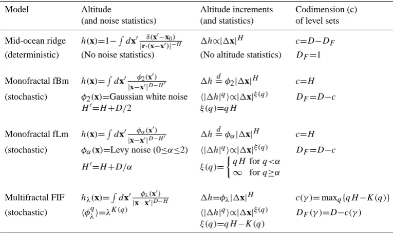
Table 1. An intercomparison between various models of the topography showing the essential similarities and differences. For additional
information about notation and definitions, see Table 2 and Sect. 3. HereD=2 for horizontal planes and the dimensionDF is the fractal
dimension of lines of constant altitude in the horizontal. The deterministic mid-ocean ridge model is represented here by a fault in unit direction vector r through the point x0. Here the variables are nondimensionalized and the height of the fault is normalized to one. Note
thatδis a Dirac delta function. The model of Turcotte and Oxburgh (1967) usesH=1/2. The monofractal fBm model is characterized by a fractional integration of orderH0of a Gaussian white noise with varianceσ2. It can also be produced by simply summing over large numbers or random Gaussian distributed faults (see Fig. 1). HereH0=H+D/2, where the extraD/2 in the exponent takes into account the scaling of the noise (Dis the dimension of space). The valueH=1/2 is compatible with the commonly cited valueDF=1.5 for the
dimension of topographic level sets. Note that=d means equality in probability distributions. The monofractal fLm model is a generalization of fBm obtained by replacing the Gaussian white noise with an independent Levy noise of indexα <2. It has diverging moments forq≥α. HereH0=H+α/2. Finally, the multifractal FIF model is a generalization of fBm and fLm. Here the multifractal noiseφλis the result of a
continuous in scale multiplicative cascade. Mathematically, it is given byφλ(x)=e0λ(x), where the generator0λ(x)∝ Rλ
1 dx 0 φα0(x0)
|x−x0|D−H0 is an
fLm process withH0=D(1−1/α)and a maximally skewed Levy noiseφα0. The resultingφλis multiplicative because it is an exponentiation
of the additive process0λ.
Model Altitude Altitude increments Codimension (c)
(and noise statistics) (and statistics) of level sets
Mid-ocean ridge h(x)=1−Rdx0 δ(x0−x0)
|r·(x−x0)|−H 1h∝|1x|H c=D−DF
(deterministic) (No noise statistics) (No altitude statistics) DF=1
Monofractal fBm h(x)=R
dx0 φ2(x0)
|x−x0|D−H0 1h
d
=φ2|1x|H c=H
(stochastic) φ2(x)=Gaussian white noise h|1h|qi∝|1x|ξ(q) DF=D−c
H0=H+D/2 ξ(q)=qH
Monofractal fLm h(x)=R
dx0 φα(x0)
|x−x0|D−H0 1h d
=φα|1x|H c=H
(stochastic) φα(x)=Levy noise (0≤α≤2) h|1h|qi∝|1x|ξ(q) DF=D−c
H0=H+D/α ξ(q)=
qH forq<α
∞ forq≥α
Multifractal FIF hλ(x)= R
dx0 φλ(x0)
|x−x0|D−H 1h=φλ|1x|H c(γ )=maxq{qH−K(q)}
(stochastic) hφλqi=λK(q) h|1h|qi∝|1x|ξ(q) DF(γ )=D−c(γ )
ξ(q)=qH−K(q)
scale invariance is the fractional Brownian motion (fBm) model of topography (Mandelbrot, 1975). In this model, to-pography is obtained by fractionally integrating a Gaussian white noise (see Table 1). In comparison, the fractionally integrated flux (FIF) model (Schertzer and Lovejoy, 1987) can be viewed as a multifractal generalization of fBm: it is obtained by replacing the Gaussian white noiseφ (with no particular relation between different scales) with a scaling multifractal noiseφλ (i.e. with long range statistical depen-dencies). This multifractal noise is the result of a cascade (see Sect. 3.1), which is a scale invariant random multiplica-tive process (Table 1). All of the models must be strongly anisotropic to be realistic.
1.4 Objectives of the present study
For more than half a century, scaling has been a feature of many topographic models. With the advent of fractals in the
Today, the scale invariance symmetry principle – having been identified with unrealistic and restrictive special cases (i.e. isotropic monofractals) – is typically disregarded or else limited to small ranges of scale. Unsurprisingly, it is consid-ered to be uninteresting and unphysical. However, the history of symmetry principles shows that their power should not be underestimated. The example of the symmetry principle of energy conservation is instructive. At first confined to me-chanical energy, it was generalized at the end of the 18th cen-tury to include heat energy. As knowledge progressed, sci-entists were repeatedly faced with the choice of either aban-doning it or generalizing it. By the mid 19th century it in-cluded chemical and electrical energy and – even though as a general principle, it was initially criticized as being overly speculative and philosophical – it was proposed as a univer-sally valid physical law. In the 20th century, it continued to be generalized to include mass-energy.
In this paper, we argue that two key advances make scaling applicable to topography: the generalization from mono to multifractals and the generalization from isotropic to anisotropic scaling. Our argument is divided in two parts. In the first part of the paper, we survey and contrast vari-ous topographic models (both deterministic and stochastic), emphasizing their similar mathematical structures. We also explain, with the help of simulations, how one can obtain a wide diversity of morphologies/textures by exploiting scaling and letting the geodynamics determine the notion of scale; this is done in the framework of Generalized Scale Invari-ance (Schertzer and Lovejoy, 1985). The simulations allow us to begin the exploration of the subtle interplay between singularities, structures, statistics and overall morphologies. We also clarify some misconceptions about multifractals and multifractal variability with the help of simulations and ped-agogical examples. Among other things, we show how su-perficially conflicting monofractal results can be understood as a result of limited statistics combined with multifractal variability.
In a previous paper (Gagnon et al., 2003), we concen-trated on the mono vs. multi fractal issue in rough surface physics using topography as an example. We clearly demon-strated that on purely statistical grounds, monofractals are not sufficient to describe topography and that multifractals are needed. We elaborate on this in the second part of the paper. In addition, the use of the large topographic data sets that have become available in the last few years allows the in-vestigation of two issues which go beyond the mono versus multifractal debate.
The first issue concerns the nature of the differences be-tween continents and oceans. Continents and oceans do not have the same geological history, so that their topographies are probably the result of qualitatively different (but still pos-sibly scaling) processes. For example, the erosion on con-tinents is due to water, wind and glaciers, whereas in the oceans it has probably been due to marine currents (little ero-sion, mostly sediment deposition).
Fig. 1. Numerical simulation of Mandelbrot (1975)’s random fault
implementation of fBm. The faults are power-law shaped (see Ta-ble 1, first and second rows) and their location and orientation are randomly chosen. The simulation is done with Gaussian statistics andH=1/2, showing development with 1, 4, 16 and 256 faults (left to right, top to bottom). The Turcotte and Oxburgh (1967) model is in the upper left corner (one fault case).
The second issue concerns the multiscaling and the “global” properties of topography. More precisely, the large range of scales of this study allows us to quantify the extent of the range of topographic multiscaling and to characterize its isotropic (angle averaged) statistics with just three funda-mental exponents α,C1 andH (see Sects. 3.2 and 3.3 for
their definitions and meanings).
The rest of the paper is organized as follows. Section 2 discusses the key issues of singularities, statistics and mor-phology with many pedagogical examples, the aim of which is to convince the reader that an anisotropic scaling frame-work is potentially capable of explaining/modelling the to-pography. Section 3 introduces some notions of multifractal theory. Sections 4 and 5 present, respectively, the data sets and the analysis techniques (power spectrum and trace mo-ments) used in the present study. Section 6 is the core of the paper and presents the results of our analyses. We finally summarize our results and conclude in Sect. 7.
2 Singularities and morphology
2.1 A survey of scaling models of topography
of scale invariant basis functions, i.e. mathematical singu-larities. Perhaps the most famous such singular model is the Turcotte-Oxburg model for the variation of altitude as a function of distance from mid-ocean ridges (Turcotte and Oxburgh, 1967). Mathematically the form is indicated in Ta-ble 1 (first row) and a simulation is displayed in Fig. 1 (upper left hand corner). Mandelbrot (1975) generalized this model by making singular faults the basic shapes and then summing large numbers of faults with random centers and orientations with Gaussian distributed amplitudes. The result is a Gaus-sian process with long range (power law) correlations; Fig. 1 shows the first few construction steps. Due to the central limit theorem (the gaussian special case), a process with the same statistical properties can be produced by using singu-larities of a quite different shape. Table 1 (second row) in-dicates a model with point rather than line singularities; in this form the mathematics is more convenient for compari-son with the other singular topography models summarized in Table 1. In this case, in the limit of many faults, because all of the singularities have nearly the same amplitude (Gaus-sian variables are rarely more than a few standard deviations from the mean), the basic singularity shape is not important: we end up with a rough texture but without any more inter-esting morphologies (see Fig. 2, second row).
Notice that in Table 1, all the stochastic models are ob-tained by convolutions with singularities. Such convolutions are “fractional integrations” of orderH0(ifH0<0, it is a frac-tional differentiation). The lesson from fBm is that if we are to represent real topography by such singular models, then the statistics of the singularities must be more extreme than Gaussians so that the basic singularity shape may remain im-portant in the limit of a large number of singularities. One way to make some of the singularities always stand out is to use the fractional Levy motion model (fLm) obtained by re-placing the Gaussian noise by a Levy noise of indexα. The Levy random variables can be regarded as a generalization of the Gaussian variables to the case where the variance (sec-ond moment) is infinite; they have long probability tails such that the statistical momentsq of order q≥α diverge. Due to the (generalized) central limit theorem, sums of indepen-dent (possibly weighted) Levy variables are still Levy vari-ables. Figure 2 (third row) shows simulations of fLm. As one can see, several strong mountain peaks stand out; in fact, the strong peaks are too strong. Although far from Gaussian, real topography empirically seems to have finite variance (i.e. the probability density tail falls off faster thanx−3), so fLm can-not be a good model. Before moving on to the statistically and visually more realistic multifractal model, let’s consider the singularity shape in more detail. The shape of line (fault-like) and point singularities depends on powers of distances from either a line or a point; in order to generalize this it turns out to be sufficient to replace the standard Euclidean distances by scale functions. Let us therefore digress a mo-ment to discuss scale functions.
2.2 Scale functions and anisotropic singularities
In order to change the shape of the singularities while con-serving the basic statistical properties of the process, it turns out to be sufficient to make the replacement everywhere in Table 1:
|x−x0| → kx−x0k ; D→Del (1)
i.e. to replace the usual distance by a new “scale function” and usual dimension of spaceDby an “elliptical dimension”
Del. These new quantities satisfy the following basic scaling
equation:
kTλxk =λ−1kxk ; Tλ=λ−G ; Del=Trace(G) (2)
whereTλis a scale changing operator which reduces the scale of a vector by a factorλ. In order for the scale function to be scaling (i.e. have no characteristic scale), it must satisfy group properties, hence it must admit a generatorGas indi-cated. In the simplest “linear” case,Gis a matrix. Once all the unit vectors x1are specified, the scale equation 2 uniquely
specifies the scale of all the other vectors; all the nonunit vectors (i.e.kxλk=λ) are then generated by the action ofTλ, i.e. xλ=Tλx1(see Schertzer and Lovejoy (1985) for
techni-cal details on this Generalized Stechni-cale Invariance, GSI). The set of all vectors with scalekxk≤λis called a “ball”, denoted
Bλ; for physical scale functionsBλ must be decreasing (i.e.
Bλ0⊂Bλ for λ0<λ). We can see that if the replacements in
Eq. (1) are made in the denominators of the models in Ta-ble 1, with scale functions satisfying the scale Eq. (2) (in fact they then define the notion of scale), then the convolutions will have power law dependencies under “zooming”, i.e. the models will be scaling as long as the noises are also scaling (hence the special choices of Gaussian or Levy noises, or in the multifractal case, of multifractal noises).
To understand the relation between usual distances and generalized scales and see how to findkxkin practice, it is in-structive to do an example. To findkxk, we need to solve the fundamental Eq. (2). Consider a (real) 2-DGmatrix which in a diagonal frame is given byG=diag(Hx, Hy)(note that what follows can be generalized to complex eigenvalues or nondiagonalizable matrices). The idea is to use a nonlinear coordinate transformation to convert the initial problem, i.e. Eq. (2) withTλ=λ−G, into an equivalent problem whereG is the identity matrix:
kλ−Ix0k =λ−1kx0k (3)
where x0=(x0, y0) are the coordinates in the nonlinearly transformed space. It is easy to show that the nonlinear trans-formationx0=sgn(x)|x|1/Hx,y0=sgn(y)|y|1/Hy does the job for the real diagonal matrix considered above. Equation (3) is now easy to solve: it represents a pure isotropic scale trans-formation, hence the solution is of the form
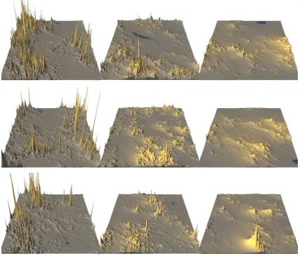
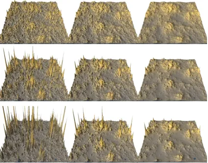
Fig. 2. Comparison of isotropic versus anisotropic (with symmetric scale functions) simulations for three different scaling models. Top row
shows scale functions. From left to right, we change the anisotropy: the left column is self-similar (isotropic) while the middle and right
columns are anisotropic and symmetric with respect toG=
0.8 −0.05 0.05 1.2
. The middle column has unit ball circular at 1 pixel, while for the
right one it has the form2(θ0)=1+0.65 cos(θ0)(in polar coordinates in the nonlinearly transformed space, see Eq. (4)). Second, third and fourth rows show the corresponding fBm (withH=0.7), fLm (α=1.8,H =0.7) and multifractal (α=1.8,C1=0.12,H=0.7) simulations.
We note that in the case of fBm, one mainly perceives textures, there are no very extreme mountains or other morphologies evident. One can see that the fLm is too extreme, the shape of the singularity (particularly visible in the far right) is quite visible in the highest mountain shapes. The multifractal simulations are more realistic in that there is a more subtle hierarchy of mountains. When the contour lines of the scale functions are close, we change the scalekxk =λrapidly over short (Euclidean) distances. For a given order of singularityγ,λγwill therefore be larger. This explains the strong variability depending on direction (middle bottom row) and on shape of unit ball (right bottom row). Indeed, spectral exponents will be different along the different eigenvectors ofG.
where r0 = (x02+y02)1/2is a radial vector in the nonlin-early transformed space and2(θ0)is an arbitrary function of the polar angle θ0 in the nonlinearly transformed space (i.e. tanθ0 = y0/x0). The nonlinear coordinate transform is then used on Eq. (4) to obtain the scale function in the original x space (as opposed to the nonlinearly transformed x0space). For the example considered, the scale function is
kxk =(2(θ0))−1 x2/Hx +y2/Hy1/2.
Fig. 3. Comparison of isotropic versus anisotropic (with “spiral” scale functions) simulations for three different scaling models. Top row
shows isotropic (left) and spiral (middle, right) scale functions. Spiral scale functions are obtained whenGhas complex eigenvalues; here
G=
0.5−1.5 1.5 1.5
. Second, third and fourth rows show the corresponding fBm (withH=0.7), fLm (α=1.8,H=0.7) and multifractal (α=1.8,
C1=0.12,H=0.7) simulations. Note how the use of spiral singularities does not affect the fBm simulations much (compare with Fig. 2).
On the other hand, spiral singularities lead to too strong singularities for the fLm, but subtle variations of mountains and plains for the multifractal.
isotropic “zooming” (blow-ups) (see the left hand column in Fig. 2). When the unit ball is a circle (or more generally aD dimensional sphere), then we obtainkxk=|x|. How-ever when the unit ball is not circular (spherical), then there will still be preferred directions. These preferred directions will be the same at all scales, the anisotropy is “trivial”. Things become more interesting as soon asGis no longer the identity. IfGis a diagonal matrix, then the singularities kxk−γ (where γ is the order of singularity, see Sect. 3.1) are quite different in different directions and the resulting
case, the anisotropy depends not only on scale but also on the location. This allows for spatially varying morphologies. In this case, the linear GSI discussed above is simply a locally valid approximation.
2.3 Spurious breaks in the scaling
In spite of the systematic finding of scaling or near ing statistics, many geophysicists reject all wide range scal-ing, often because of their conviction that geomorphologic processes are scale dependent: they consider a priori that the scaling is broken. For example, Herzfeld et al. (1995); Herzfeld and Overbeck (1999) have attempted to demon-strate broken scaling by estimating power spectra and var-iograms on a few bathymetry transects which they showed to have poor scaling. Rather than giving a purely theoreti-cal explanation as to why their results are not surprising and how they could be compatible with the scaling hypothesis, let us consider a simulation of their transect (see Fig. 4). The figure compares the energy spectra of two individual tran-sects as well as the ensemble average over all the trantran-sects. One of the transects passes through “Mt. Multi” (the high-est peak in the range), another through a randomly chosen transect not far away. One can see that the Mt. Multi scal-ing is pretty poor; a naive analysis would indicate two ranges with a break at about 10 pixels with high frequency exponent
β≈2.5, low frequencyβ≈1.5. Clearly this significant break has nothing to do with the scaling of the process (which is perfect except for finite element effects affecting the high-est factor of two or so in resolution). In comparison, the randomly chosen transect has better scaling, but withβ≈2. On the other hand, the isotropic (i.e. angle averaged) spec-trum averaged over an infinite ensemble of realizations has
β≈2.17. Even the average over the transects shows signs of a spurious break at around 16 pixels (the scale where the north-south and east west fluctuations are roughly equal in magnitude, the “sphero-scale”); this explains why the theo-retical line does not pass perfectly through the curve corre-sponding to the average of the transects. Obviously, had we chosen a different random seed for the simulation, the results for the individual transects would have been different (even the average over the transects would have been a bit differ-ent), see the example in the next section.
Conclusions about broken scaling in Fig. 4 are therefore unwarranted. The most important reason to explain apparent scaling breaks is that scale invariance is a statistical symme-try, i.e. defined on an infinite ensemble (see Sect. 3.2). This means that scaling is almost surely broken on every single re-alization, hence it is important to have a large data base (i.e. large range of scales, many realizations) to average fluctua-tions and approximate the theoretically predicted ensemble scaling. In fact, due to the singularities of all orders (see Sects. 2.1 and 3.1) the realization to realization variability of multifractals is much greater than that of classical stochas-tic processes; for example, rare (extreme) singularities are
Fig. 4. Figure showing a bathymetry simulation (with α=1.9,
C1=0.12 andH=0.7). The energy spectra of the transect
pass-ing through “Mt. multi” (the highest peak in the simulation) and through another (randomly chosen) transect are shown as well as the ensemble over all the transects. We can see that the scaling in the transect containing the extreme event “Mt. Multi” is clearly bro-ken, even though the ensemble scaling is very good. Figure taken from Lovejoy et al. (2005).
produced by the process yet they are almost surely absent on any given realization. This means that they do not have the property of “ergodicity”. What may be nothing more than normal multifractal statistical variability can thus eas-ily be interpreted as breaks in the scaling. The second rea-son for erroneously concluding that the scaling is broken is the assumption that the scaling is isotropic. If the scaling is anisotropic, then breaks in the scaling on 1-D subspaces (transects) do not imply anything about the scaling of the full process.
2.4 Apparent nonstationarity, inhomogeneity, parameter variations... or simply random exponents?
Fig. 5. 1024×1024 self-similar multifractal simulation with some trivial anisotropy and parameters α=1.9, C1=0.12 and H=0.7.
The spectral exponent isβ=1+2H−K(2)=2.17.
realization – often leads to claims of statistical inhomogene-ity/nonstationarity. In the case of multifractals, it is partic-ularly tempting to invoke statistically inhomogeneous mod-els (corresponding to different physical processes in different locations) since their occasionally strong singularities often stand out from a background of more homogeneous noise. However, the basic multifractal processes are statistically sta-tionary/homogeneous in the strict sense that over the region over which they are defined (which is necessarily finite), the ensemble multifractal statistical properties are independent of the (space/time) location (and this, for any spectral slope
β). Rather than discussing this at an abstract level, let us see what happens when we analyse a self-similar 1024×1024 multifractal simulation (Fig. 5). Figure 6 shows the compen-sated (i.e. k2.17E(k)), isotropic spectrum obtained by inte-grating the Fourier modulus squared over circles of radiusk
in Fourier space. The low frequencies are quite flat, indicat-ing that the simulation has roughly the expected ensemble spectrum. At high frequencies, there is a drop-off which is an artifact of the numerical simulation techniques. We can now consider the “regional” variability in the spectral ex-ponentβ by dividing the simulation into 8×8 squares, each with 128×128 pixels. Figure 7 (left) shows the histogram of the 64 regression estimates of the compensated spectra: the mean is close to zero as expected, but we see a large scat-ter implying that there are some individual regions havingβ
as low as 1.2, some as high as 2.7; the standard deviation is±0.3. As we shall see later, this would imply a random
Fig. 6. Compensated power spectrum (i.e.k2.17E(k)) of the multi-fractal simulation in Fig. 5. The extreme factor of 2 in wavenumber falls off too rapidly: this is an artifact due to the difficulty of dis-cretizing singularities on numerical grids.
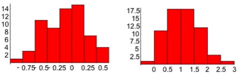
Fig. 7. On the left, we have a histogram of the compensated
spec-tral exponent (1β=β−βtheo=β−2.17) values obtained after
divid-ing Fig. 5 into 64 128×128 squares, and computing the isotropic power spectrum in each square (the vertical axis is the number of occurences out of the total of 64). In each case, we fit the slope to the lowest factor of 16 in scale (we remove the highest factor of 4 due to numerical artifacts at the highest wavenumbers). On the right, we have a histogram of the log10E1(E1is the spectral
pref-actor,E(k)=E1k−β) showing a variation of a factor of about 1000
from the smoothest to the roughest subregion.
variation in local estimates of H of ±0.3/2=±0.15, which is of the order of the difference observed between continents and oceans (see Sect. 6.1.1), although this spread inβ will decrease as the size of the data set increases. Similarly, use of the monofractal formulaDF=7/2−β/2 would lead to a corresponding wide spread of “local” fractal dimension.
In Fig. 7, we can also see the large variations in the log prefactors (i.e. log10E1, whereE(k)=E1k−β). If this is
re-gions has about 103times the variance of the smoothest re-gion. While it would obviously be tempting to give different interpretations to the parameters in each region, this would be a mistake. Note that this does not imply that the roughest and the smoothest would be associated with identical ero-sional, orographic or other processes. The point is that in a fully coupled model involving various geodynamical pro-cesses, all the processes would be scaling and would have correlated variations. Figure 4 also demonstrates the fact that if data from special locations (such as near high mountains) are analysed that we may expect systematic biases in our statistics and parameter estimates. These conditional statis-tics are discussed quantitatively and theoretically in Lovejoy et al. (2001b). This underlines the need for coupled multi-fractal processes, possible through the use of a state vector and vector mulitfractal processes (based on “Lie cascades” (Schertzer and Lovejoy, 1995; Lovejoy et al., 2001b)).
3 Properties of multifractals
3.1 Multifractal processes and scale invariance
In Sect. 2, we discussed the crucial role of singularities. Multifractals allow singularities of various orders to be dis-tributed over fractal sets with varying fractal dimensions (rather than a unique dimension as for monofractal processes such as fBm, fLm). In this section we show how the key (multiplicative part) of the process can be viewed as a step by step build-up of variability from an initially uniform state. This multiplicative process is often called a “cascade”; it is the generic multifractal process.
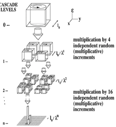
Cascades are phenomenological models of processes which have the following properties: (1) They have a scale by scale conserved quantity; it is this conserved quantity that is modulated by nonlinear interactions as it goes down the scales. (2) Localness in Fourier space, i.e. structures of a certain size interact most strongly with structures of not too different sizes. (3) Scale invariance; over a range of scales, the mechanism doesn’t change. To illustrate these points and show how cascades are related to multifractals, let us con-struct a very simple cascade, theα-model (e.g., Schertzer and Lovejoy, 1985). This model is very close to the model of de Wisj (1951) for the distribution of mineral ores.
To help the reader through this section, a summary of our notation is provided in Table 2. Consider a certain quan-tity φ uniformly distributed in a D dimensional space of sizeLD (to apply this to topography, just replaceDwith 2). Supposing that the system (including its surroundings) has a very high number of degrees of freedom, we want to know how the quantityφwill be distributed in theDdimensional space after undergoing a large number of nonlinear interac-tions with the whole system. Consider a simple discrete scale ratio model (α-model); the continuous in scale extension is given in Table 1. The first step is to specify an integer ratio
Fig. 8. Example of a 2-D cascade process. At each step of the
cas-cade, the noiseφ(represented byε in the above picture) in each square is multiplied by a random increment, here given by the prob-abilistic law in Eq. 5. Figure taken from Schertzer and Lovejoy (1985).
φ
λ(x)
λ
γ1λ
γ2L/λ
Set 2
Set 1
x
Fig. 9. Illustration of Eq. (6) using a 1-D example of a cascade. For
different thresholdst1=λγ1andt2=λγ2 (withγ2>γ1), the
corre-sponding sets (defined byφλ>t) have different fractal dimensions
(DF(γ2)<DF(γ1)) or fractal codimensions (c(γ2)>c(γ1)).
of scalesλ0=L/ l0(typically 2); we then separate the initial
Table 2. Summary of notation and important quantities.
Symbol Quantity Definition Reference1
l Length scale — Eq. (6)
L Maximum length of a process — Eq. (6)
λ Resolution λ=L/ l Eq. (6)
Tλ Scale changing operator Tλ=λ−G Eq. (2)
G Generator D×Dmatrix or operator Eq. (2)
D Dimension of space — Sect. 3.1
DF Fractal dimension of a set — Sect. 3.1
c Codimension of a set c=D−DF Sect. 3.1
γ Order of singularity — Sect. 3.1
t Threshold t=λγ Fig. 9
φλ Scaling multifractal noise — Sect. 3.1
K(q) Moment scaling function K(q)=maxq{qγ−c(γ )} Sect. 3.2
1hλ Height increment h(x+λ−11x)−h(x) Eq. (9)
α Degree of multifractality 0≤α≤2 Sect. 3.2
C1 Sparseness of the mean singularity 0≤C1 Sect. 3.2
H Degree of smoothing — Sect. 3.3
ξ(q) Structure function exponent ξ(q)=qH−K(q) Sect. 3.3
β Spectral exponent β=1+ξ(2) Sect. 5.1
1Specifies the section or the equation where the symbol is defined or explained.
Pr(µ=λγ0+)=λc0
Pr(µ=λγ0−)=1−λc0 (5)
where µ is a “multiplicative increment” multiplying φ,
γ+>0,γ−<0 are positive/negative singularities andcis the
codimension of the space occupied byφ. The de Wisj (1951) model is obtained by restricting this model so that the mean
µ=1 on each cascade step (microcanonical conservation), whereas the above “α-model” only enforces this conserva-tion on the ensemble average (canonical conservaconserva-tion). It is now known that microcanonical conservation results in much less variable processes and is generally unrealistic. Equa-tion (5) corresponds to an increase (λγ+
0 ) or a decrease (λ
γ−
0 )
inφ. Note that the parametersγ+andγ−cannot be chosen
independently if we wantφto be conserved, as prescribed by assumption (1). Afternsteps,φis broken up into(λD0)n
cubes and the succession of decreases/increases leads to a highly heterogeneousφ. In fact, it leads to a whole hierar-chy of singularitiesγi with values betweenγ−n≤γi≤γ+n(see
Fig. 8). The cascade just described is artificial because of its discrete in scale nature. Letting the scale ratioλ0 become
continuous (i.e.λ0→1;n→∞;λ=λn0=constant), we obtain
(Schertzer and Lovejoy, 1987):
Pr(φλ≥λγ)∼λ−c(γ ) (6)
where the notation φλ stands for φ at the scale L/λ, λγ is the threshold corresponding to the singularity γ and
c(γ ) is a nonlinear convex function called the codimen-sion function. Equation (6) means that the set defined by the condition φλ≥λγ has a (fractal) codimension given by
c(γ )=D−DF(γ ), whereDF(γ )is the fractal dimension of the set (see Fig. 9). Thus, the initial uniformly distributed quantityφis now a hierarchy of interwoven sets, one for each threshold, each of them having a different fractal codimen-sion: a multifractal. In comparison, a monofractal process has a unique fractal dimension for all thresholds. The scale by scale conserved multifractalφλ will be referred to as a multifractal noise.
3.2 Moment scaling function and universal multifractals One way to characterize the statistics of stochastic processes is via probability distributions. For a multifractal process, the probability distribution is a power law, as given in Eq. (6). Equivalently, we can characterize the statistics of stochastic processes by the moments of the probability distribution (Pr), hxqi=R∞
0 dPr x
q. In the case of multifractal processes, this gives (Schertzer and Lovejoy, 1987, 1991):
hφλqi =λK(q) (7)
where q is the order of the moment andK(q)is a nonlin-ear convex function. K(q)characterizes the scaling of the moments of the multifractal noise, hence it is called the “mo-ment scaling function”. If the multifractal noise is conserved with scale (i.e.hφλi=1), then it implies thatK(1) =0; for a nonzero processK(0)is also trivially equal to zero. K(q)
andc(γ )are related to each other via a Legendre transform,
moments, we fix a momentqand then take the averagehφqλi; depending onq, certain orders of singularities dominate the average (for example, a high q favors strong singularities compared to weaker ones). The bottom line is that analyz-ing a certain moment is equivalent to probanalyz-ing a certain sin-gularity (a one to one correspondence given by the Legendre transform), but it is usually more convenient to do moments analysis.
A priori, the only constraint onK(q)is that it must be con-vex, which implies that an infinite number of parameters are generally needed to describe it; without further constraints, it would not be manageable. Schertzer and Lovejoy (1987, 1991) have shown that there exists a class of stable and attrac-tive multifractal processes called “universal multifractals”, which are thus generic outcomes of multifractal processes independent of many of the details (see Schertzer and Love-joy (1997) for the debate about this issue). Here we postulate the functional form given in Eq. (8) on theoretical grounds (it can be viewed as a consequence of a “multiplicative central limit theorem”), but we will see in Sect. 6.2.4 that the esti-mated error with thisK(q)is quite low, so that this can also be viewed as a way of parametrizing the data. The universal
K(q)is given by the following functional form:
K(q)= C1
α−1 q α−q
(8) whereαandC1are the two basic parameters characterizing
the scaling properties of the multifractal noiseφλ. The pa-rameterαis the degree of multifractality and varies from 0 to 2, whereα =0 is the monofractal case andα =2 is the log-normal case. This parameter describes how rapidly the fractal dimension of sets at different thresholds vary as they leave the mean singularity. It is not very intuitive; the ac-companying simulations (see Fig. 10) may be the best way to visualize the effect of varyingα. The parameterC1is the
fractal codimension of the set giving the dominant contribu-tion to the mean (q=1) and is bounded below by zero. The valueC1=0 implies that the set giving the dominant
contri-bution to the mean is space filling (i.e. its fractal dimension is equal to that of the embedding space), so it can be interpreted as quantifying the sparseness of the mean field. Again, com-pare Figs. 10–11 or see the simulations of Fig. 12 to see the effect of varyingC1on a multifractal process.
3.3 Fractionally integrated flux model
We have discussed (Table 1) several scaling models and have seen that fBm/fLm are additive, being the result of a gen-eral scaling linear operator (a fractional integral/derivative) acting on a basic scaling noise (Gaussian and Levy, re-spectively). These lead to exponent functions linear in the moment q (e.g. the structure function exponent ξ(q), see Eq. (10)). We saw that in order to obtain more general scal-ing behaviour, we could retain the fractional integration of a noise, choosing the basic noise instead to be the result of
a multiplicative process (the cascade). We saw that the cas-cade generates a scale by scale conserved noiseφλ charac-terized by a moment scaling functionK(q)(a convex func-tion with the constraintsK(0)=0,K(1)=0). The spectrum of the conserved noise has exponentβ=1−K(2)<1. So to characterize topography (having β≈2), we clearly need an extra fractional integration; this is the Fractionally Integrated Flux model described in Table 1. The fractional integration of the multifractal noise leads to the following statistics for the height increments (Schertzer and Lovejoy, 1987, 1991):
1hλ=λ−Hφλ (9)
where1hλ ≡1h(1x)=h(x+1x)−h(x)(with|1x| =
L/λ) are the height fluctuations a distance l = L/λapart (as usual, the anisotropic generalization is obtained using |1x| → k1xk). The parameterHcan be interpreted as a de-gree of smoothness where higherH means smoother fields. Figures 10–14 show examples of changing the degree of frac-tional integrationHin conjunction withα,C1.
As mentioned earlier, statistical moments analysis is more convenient than direct height analysis. We take theqth power on both sides of Eq. (9) and then the ensemble average which leads to
h|1hλ|qi =λ−ξ(q) ; ξ(q)=qH −K(q) (10) whereh|1hλ|qiis theqth order structure function andξ(q) is the corresponding scaling exponent. The special case
q=2 corresponds to ensemble averaged variograms. Equa-tion (10) models the statistical properties of topographic height increments and is the culminating point of the mul-tifractal FIF model. Note that if the multiscaling noise φλ in Eq. (10) is replaced with a noise with no particular rela-tion between scales (i.e.K(q)=0) such as a Gaussian white noise, then we obtain fractional Brownian motion (see Ta-ble 1 for a comparison). This last comment is particularly important when it comes to data analysis and will help us to distinguish between multifractal and monofractal behav-ior (see Sect. 5.2). It also helps to clarify the advantage of multifractals over monofractals: the multifractal noiseφλis much more variable than Gaussian white noise, leading to a much better characterization of extreme events, such as very high mountains.
An important caveat is in order at this point. The 2-D anal-yses in this study are restricted to isotropic (i.e. self-similar) statistics. By isotropic analysis, we mean that the resolution
Fig. 10. Isotropic (i.e. self-similar) multifractal simulations showing the effect of varying the parametersαandH (C1=0.1 in all cases).
From left to right,H = 0.2, 0.5 and 0.8. From top to bottom,α=1.1, 1.5 and 1.8. AsH increases, the fields become smoother and as
αdecreases, one notices more and more prominent “holes” (i.e. low smooth regions). The realistic values for topography (see Table 5) correspond to the two lower right hand simulations. All the simulations have the same random seed.
H. We thus argue that isotropic statistics do not vary much from place to place even if morphologies/textures vary appre-ciably (see Figs. 2–3 and Figs. 12–14 for some isotropic vs anisotropic simulations). For additional simulations and “fly-bys” of topography and other geophysical fields, we refer the reader to the following website: http://www.physics.mcgill. ca/∼gang/multifrac/index.htm. Additional simulations
ex-ploring anisotropic topographies may also be found in Love-joy et al. (2005).
4 Data sets
In this study, several Digital Elevation Models (DEMs) that span various ranges of scales are analyzed. DEMs are grid-ded representations of topography. They are constructed via
various techniques including stereo-photography and in situ measurements of altitude (often combined using complex jective analysis techniques) and are then gridded so as to ob-tain a height field. They are essentially characterized by their horizontal and vertical resolutions.
quan-Fig. 11. Same as quan-Fig. 10, but withC1=0.3. The effect of increasingC1is to make high areas much more sparse. It is interesting to note the
presence of isolated high peaks in very flat areas.
titatively in Sect. 6.2.2. Another problem is oversampling, which results when the altitude is sampled more frequently than is warranted by the source data; this implies an artifi-cially smooth DEM at the highest wavenumbers. The cur-vature of the Earth can also be a problem; because DEMs are gridded representations of the topography, it is necessary to project a sphere on a plane to produce the DEM. When averaging many transects at different latitudes, this can in-duce changes in the highest wavenumbers. The main point is that each DEM has its own characteristics and problems, but these problems usually manifest themselves at the highest or smallest wavenumbers. On the other hand, different physical mechanisms would induce clean breaks in the scaling.
Four different DEMs are analyzed in this study. We refer the reader to Table 3 for their individual characteristics (res-olution, vertical discretization, etc.) and to Figs. 15–17 for the regions analyzed on each of them. The data sets are:
ETOPO5 (global topography including bathymetry) (Data Announcement 88-MGG-02, 1988); GTOPO30 (global con-tinental topography) (Land Processes Distributed Active Archive Center, 1996); United States (DEM of the United States) (United States Geological Survey, 1990); Lower Sax-ony (DEM of a 3 km×3 km section of Lower Saxony, con-structed with the help of the High Resolution Stereo Camera Airborne (Wewel et al., 2000)).
5 Analysis techniques
in-Fig. 12. Isotropic (i.e. self-similar) multifractal simulations showing the effect of varying the parametersC1andH (α=1.8 in all cases).
From left to right,H=0.2, 0.5 and 0.8. From top to bottom,C1=0.05, 0.15 and 0.25. AsH increases, the fields become smoother. When C1is low, field values are close to the mean everywhere; whenC1is large, all values are below the mean except in some specific locations
where they are very large. The values closest to the data (see Table 5) correspond to the middle row (middle and right columns).
Table 3. Characteristics of the DEMs and regions studied.
Data sets Horizontal Vertical Numbers of Length of
resolution discretization transects analyzed transects (km)
ETOPO5 5’ (≈10 km) 1 m 500 and12160 40 000
GTOPO30 30” (≈1 km) 1 m 1225 4096
U.S. 90 m 1 m 2500 5898
Lower Saxony 50 cm 10 cm 3000 and2500 3 and20.512
1Analysis with constant angular resolution. 2Analysis on treeless region.
finity of independent samples are needed to obtain accurate scaling. In this study, all samples (transects or squares) ana-lyzed are correlated because they come from the same region and from the same unique Earth. This means that the aver-ages in this study are at best approximations to the required ensemble averages.
5.1 Analysis of the height: Power spectra
Fig. 13. Anisotropic (self-affine) multifractal simulations with varyingC1andH (α=1.8 in all cases). From left to right,H=0.2, 0.5 and
0.8. From top to bottom,C1=0.05, 0.15 and 0.25. The scale changing operator isG=
Hx 0
0 Hy
(withHx=1.2 andHy=0.8) and the
sphero-scale is 1 pixel. Transects in the up-down (y) or left-right (x) directions do not have the same spectral exponents: they are related through the ratio(βx−1)/(βy−1)=Hx/Hy, whereβx,βyare the 1-D spectral exponents in thex,ydirections, respectively.
angle averaging is used; this increases the spectral exponent by 1). Before estimating power spectra, we removed linear trends (in 1-D analyses) and we used Kaiser windows (in 2-D in analyses) to avoid problems at the lowest wavenumbers. The (isotropic) power spectrum of a scaling process is given by
E(k)∝ |k|−β (11)
where k is the wavenumber andβ=1+ξ(2)=1+2H−K(2)
is the spectral exponent. It can be seen that the simple scaling result is recovered ifK(2)=0. The power spectrum is only a second order moment, so that this method alone cannot be used to distinguish between simple and multiscaling. 5.2 Analysis of the noise: Trace moments
As can be seen from Table 1, the fBm and FIF models may be hard to distinguish because they both share a
convolu-tion characterized by the exponentH. A better way to dis-tinguish them is to consider their noiseφ, which has com-pletely different properties: a delta correlated Gaussian white noise for fBm viz. a scaling singular multifractal noise for FIF. We are therefore lead to the use of “trace moments” (which directly characterize φ) so that the distinction will be far more apparent. The first step is to obtainφfrom the height increments: in principle this involves removing the
Fig. 14. Same simulations as Fig. 13, but with a sphero-scale equal to 64 pixels instead of 1 pixel. We still have left-right “mountain chains”
but at scales smaller than 64 pixels, we have up-down “ridges”. This is what a typical pixel of Fig. 13 would look like if blown up by a factor of 64.
value of wavelet coefficients at the finest available resolution (Muzy et al., 1993; Audit et al., 2002). (Technical note: Be-cause of the insufficient dynamical range of the DEMs (see Sect. 4), many spurious zero gradients are present in the an-alyzed transects. Those zero gradients particularly affect the lowq statistics, so they are eliminated by a fractional inte-gration of orderH=0.1 (a filtering in Fourier space with a power law), which is a scale invariant smoothing.) After the removal ofλ−Hin Eq. (9), we are left with only the underly-ing noiseφλ. The next step is to study the scaling of the sta-tistical moments ofφλand compare them with Eq. (7). To do this, we normalizeφλso that the ensemble average of all the samples ishφλi=1. Then spatial averaging is performed over sets (lines or squares) of sizel=L/λ, theqth power is taken and the average over all data available is taken: this gives the moments of the normalized noise for a given value of
q. This procedure is performed for different values ofq and
K(q)is determined from the logarithmic slopes;
multiscal-ing is verified if we find a nonlinearK(q). For the monofrac-tal fBm, the moments of the normalized flux are equal to 1 for allq, i.e.K(q)=0. In other words, if after doing the frac-tional differentiation we get a Gaussian white noise (with no scale/resolution dependence, i.e.K(q)=0), the data are com-patible with a fBm process.
studied using numerical simulations (Lavall´ee et al., 1993). With the large topography data sets available in this study, the scale range is so large that this is not so difficult. In any case, functional box-counting (Lovejoy and Schertzer, 1990) and generalized structure functions (Lavall´ee et al., 1993; Weis-sel et al., 1994) also clearly indicate multiscaling over wide ranges of scale; breaks are indeed confined to the highest wavenumbers of each data set.
6 Results and discussion
6.1 Analysis of continents and oceans
The morphologies of continental and oceanic topography are clearly different. In the scaling framework, these differences can arise in several ways. One effect that we already men-tioned (see Sect. 3.3) is that the anisotropy varies not only from scale to scale but also from place to place: another set of scaling exponents are needed to characterize these anisotropies. In this paper we limit ourselves to isotropic analyses (analysis of scaling anisotropy is quite difficult (e.g., Lewis et al., 1999)). For example, the 2-D spectra are an-gle integrated or in the case of trace moments we average on squares at each scale. In both cases, we “wash out” the anisotropies and consider only the isotropic statistics. We have also seen in Sect. 2 that due to their strong singularities, individual realizations of multifractals can have strong vari-ations from one region to another even though the process is strictly homogeneous, stationary (statistically translationally invariant). This means that it is not trivial to test the scaling and estimate the parameters.
The continent/ocean comparison is made using power spectra and trace moments on ETOPO5. Three 512×512 pixels squares (≈5120×5120 km) are analyzed in the case of continents and five in the case of oceans (shown on Fig. 15). The ensemble average is performed over the three (five) squares of continents (oceans) for the two methods of analy-sis.
6.1.1 Power spectrum analysis
A comparison between the averaged spectra from continents and oceans is shown on Fig. 18. According to Eq. (11), a log/log plot of the spectral energyE(k)versus the wavenum-berkshould give a straight line if the process is scaling. The spectra are fairly straight over 2 orders of magnitude, imply-ing that they are scalimply-ing over that range. There is a break in the scaling at approximately 50 km, which is probably due to oversampling. Note that there is a systematic difference in the slope of the spectra: βcontinents=2.09 (c.f.β≈2 (Vening
Meinesz, 1951)) andβoceans=1.63, in agreement with
Berk-son and Matthews (1983) (β≈1.6−1.8) but less than the val-ues of Bell (1975) (β≈2), Fox and Hayes (1985) (β≈2.5) and Gibert and Courtillot (1987) (β≈2.1−2.3). The dif-ferences between the values ofβ may be a consequence of
Fig. 15. ETOPO5 data set (Data Announcement 88-MGG-02, 1988). See Table 3 for its specific properties. The white and black squares indicate the areas studied in Sect. 6.1. The white rectangle indicates the area used for the narrow strip analysis (500 transects of 40 000 km).
the fact that estimates of the spectral exponent require large amounts of data and wide ranges of scales (see Sect. 2.3). In addition, for multifractals the values ofβ in any single real-ization is random with (depending on parameters) a possibly large scatter (see Sect. 2.4). In the studies mentioned above, the analyses are on small data sets (104 compared to 106 points here), which result in “fuzzy” or even broken spec-tra, making it hard to find the scaling range. This means that the spectral exponents may not be well estimated in those studies.
6.1.2 Trace moments analysis and the universal multifrac-tal parameters
Fig. 16. U.S. part of the GTOPO30 data set (Land Processes
Dis-tributed Active Archive Center, 1996). See Table 3 for its spe-cific properties. The black rectangle indicates the area studied on GTOPO30 (1225 transects of 4096 km) and the white rectan-gle indicates the area studied on the U.S. DEM (2500 transects of 5898 km).
Table 4. Universal multifractal parameters for the conti-nents/oceans analysis.
Type of region α C1 H
Continents 1.82±0.17 0.13±0.04 0.66±0.04
Oceans 1.87±0.15 0.15±0.02 0.46±0.03
Continental margins 1.80±0.05 0.12±0.02 0.77±0.02
filling) support corresponding toC1 = 0. In Fig. 19, the β-model would give nonzero slopes that would vary linearly withq(theK(q)’s in Fig. 20 would followK(q)=C1(q−1)).
We see below that this is also incompatible with the data. We may also note that the fLm is not compatible with the data ei-ther; this is because statistical moments substantially larger thatq=2 have no obvious anomalous behaviours (visible as a “multifractal phase transition”, i.e. a discontinuity in the derivative ofK(q)atq =2).
The slopes of the trace moments for eachq yieldK(q); from this we estimate the parametersαandC1for continents
and oceans. Equation (8) is used to fit the curves on Fig. 20 and the results are shown in Table 4. The errors in the table are equal to one standard deviation of the individual values of
αandC1for continents and oceans. By taking into account
the error, we conclude that continents and oceans may have the sameαandC1.
Fig. 17. Lower Saxony DEM (Wewel et al., 2000). See Table 3
for its specific properties. The global analysis of Sect. 6.2 is done on the upper half of the above DEM to avoid contamination from man-made structures. The total area covered is 3000 transects of 3000 m. The small white rectangle (500 transects of 512 m) is the treeless section analyzed and compared to the full DEM analysis.
-7.0 -6.5 -6.0 -5.5 -5.0 -4.5 -4.0
log10k (cycles/m)
4 5 6 7 8 9 10
log
10
E(k) (m
3 )
Continents Oceans
Fig. 18. Log/log plot of the spectral energy versus the wavenumber
-0.5 0.0 0.5 1.0 1.5 2.0 2.5 3.0 log10λ
-0.2 -0.1 0.0 0.1 0.2 0.3 0.4 0.5 0.6 0.7 0.8 0.9
log
10
<
φλ(d)
q >
0.0 0.5 1.0 1.5 2.0 2.5 3.0
log10λ -0.2
-0.1 0.0 0.1 0.2 0.3 0.4 0.5 0.6 0.7 0.8 0.9
Fig. 19. Log/log plot of the normalized trace moments versus the
scale ratioλ=L/ lfor continents (left) and oceans (right), both with
L=5120 km. The values of the exponentqof each trace moments
are, from top to bottom, 2.18, 1.77, 1.44, 1.17, 0.04, 0.12 and 0.51.
0.0 0.5 1.0 1.5 2.0
q -0.05
0.00 0.05 0.10 0.15 0.20 0.25
K(q)
Continents Oceans
Fig. 20. Plot of the moment scaling functionK(q)as a function of the momentq (circles correspond to continents and squares to oceans).
The values ofαandC1combined withβyield the values
of H for continents and oceans (see Eq. 11 and following discussion). The results are shown in Table 4. TheH value for oceans is quite near the commonly cited value ofH=1/2 (e.g., Bell, 1975), but theH value for continents is system-atically larger. This can also be seen on the scatter plots of Figs. 21 and 22, where there is a clear stratification of the
H values but not of the αandC1 parameters (where there
is only a certain spread). This result is compatible with the hypothesis that the statistics of the noiseφλ (determined by
αandC1) are the same for continents and oceans, but the
height statistics (see Eqs. 7 and 10) are different becauseH
is different. The higher value ofH for continents means that they are smoother than the seafloor. It means that the under-lying physical mechanisms responsible for the values ofα
andC1, whatever they are, may be the same for continents
1.0 1.2 1.4 1.6 1.8 2.0 2.2 2.4
α 0.3
0.4 0.5 0.6 0.7 0.8 0.9 1.0
H
Continents Oceans
Continental margins
Fig. 21. Scatter plot of the parameters (α,H) for the three different types of region (circles, stars and X’s represent continents, oceans and continental margins respectively).
and oceans. On the other hand, the mechanisms responsi-ble forH (related to erosion-like processes) are likely to be different. It also means that the simple dimensional analysis (withH=1/2) proposed by Lovejoy et al. (1995) does not hold on continents.
6.1.3 Continental margins
In addition to the continents and oceans, it is also of interest to consider the statistics of the transition region from one to the other, i.e. the continental “margins”. These regions have very large topographic gradients and may therefore have a differentH. Also, since Sect. 6.2 deals with the global anal-ysis of topography, i.e. the combined analanal-ysis of continents and oceans (on the same transect), this region is important. So we apply the same procedure as for continents and oceans on 5 square regions that include a continental margin (not shown on Fig. 15, but very near the squares already drawn). The final universal parameters are given in Table 4. As can be seen, once again theαandC1 parameters do not differ
significantly from those of continents and oceans, but theH