A new algorithm for detecting cloud height using OMPS/LP measurements

(1)

www.atmos-meas-tech.net/9/1239/2016/ doi:10.5194/amt-9-1239-2016

A new algorithm for detecting cloud height using OMPS/LP

measurements

Zhong Chen1, Matthew DeLand1, and Pawan K. Bhartia2

1_{Science Systems and Applications, Inc., 10210 Greenbelt Road, Suite 600, Lanham, Maryland 20706, USA} 2_{NASA Goddard Space Flight Center, 8800 Greenbelt Road, Greenbelt, Maryland 20771, USA}

Correspondence to: Zhong Chen ([email protected])

Received: 30 July 2015 – Published in Atmos. Meas. Tech. Discuss.: 2 October 2015 Revised: 9 March 2016 – Accepted: 11 March 2016 – Published: 23 March 2016

Abstract. The Ozone Mapping and Profiler Suite Limb Pro-filer (OMPS/LP) ozone product requires the determination of cloud height for each event to establish the lower boundary of the profile for the retrieval algorithm. We have created a revised cloud detection algorithm for LP measurements that uses the spectral dependence of the vertical gradient in ra-diance between two wavelengths in the visible and near-IR spectral regions. This approach provides better discrimina-tion between clouds and aerosols than results obtained using a single wavelength. Observed LP cloud height values show good agreement with coincident Cloud-Aerosol Lidar and In-frared Pathfinder Satellite Observation (CALIPSO) measure-ments.

1 Introduction

The Ozone Mapping and Profiler Suite Limb Profiler (OMPS/LP) is one of three OMPS instruments on board the Suomi National Polar-orbiting Partnership (S-NPP) satellite (Flynn et al., 2007). S-NPP was launched in October 2011, into a sun-synchronous polar orbit. The local time of the ascending node of the S-NPP orbit is 13:30. The LP in-strument collects limb-scattered radiance data and solar ir-radiance data on a 2-D charge coupled device (CCD) ar-ray over a wide spectral range (290–1000 nm) and a wide vertical range (0–80 km) through three parallel vertical slits. Each slit provides a 1.85◦vertical field of view (FOV) cor-responding to a 112 km vertical extent at the tangent point. The FOV of each slit is separated horizontally by 250 km in the cross-track direction. The OMPS/LP produces three ozone profiles every 19 s along the orbit track, which

cor-responds to a sampling distance of about 150 km (approx-imately 1◦ latitude). OMPS/LP has been operating contin-uously since April 2012, collecting approximately 160–180 measurements (events) per orbit for each of the three slits and each of the 14–15 orbits per day. Jaross et al. (2014) pro-vide more details about the OMPS/LP instrument design and capabilities.

Retrieval of ozone profiles from limb-scattering measure-ments becomes extremely difficult in the presence of tropo-spheric clouds, because these clouds shield the signal from the lower atmosphere and also reflect a part of the incom-ing radiation back to space. Due to the potential bias in the retrieved profiles from clouds, the OMPS/LP retrievals are based on a cloud-free assumption. Thus, the current ozone retrieval algorithm applied to LP measurements is designed to identify cloud height (if present) for each event and to ter-minate the retrieval 1 km above this height.

(2)

1240 Z. Chen et al.: A new algorithm for detecting cloud height

change in the vertical gradient of visible or near-infrared ra-diances. Clouds appear as either faint or sharp discontinu-ities in the reflected sunlight radiance vertical profiles. How-ever, aerosol layers can also cause relatively abrupt changes in the radiance profile at visible and IR wavelengths, so this approach cannot always differentiate between tropospheric cloud and aerosols.

This paper describes a revised approach to cloud-top height detection using OMPS/LP measurements, based on the spectral dependence of the vertical gradient in radiance between two wavelengths. The approach is simple to imple-ment. It is capable of distinguishing between aerosols and cirrus clouds in many cases. We show that the performance of this approach is consistent with Cloud-Aerosol Lidar and Infrared Pathfinder Satellite Observation (CALIPSO) results for quasi-coincident orbits in individual cases, as well as for a larger statistical comparison.

2 Algorithm design

The new gradient-based LP cloud detection algorithm as-sumes that clouds produce a larger gradient in radiances than aerosols. Because of the different size distributions between aerosol particles and cloud hydrometeors, their scattering of incoming solar radiation shows a different behavior. At UV and shorter visible wavelengths, Rayleigh scattering reduces the contrast between cloudy and clear pixels. This contrast increases with longer visible and near-IR wavelengths. Since aerosol particles are smaller, their increase in brightness is less pronounced for the same change in wavelength, so the increase in contrast for aerosols is not as large as for clouds. We define the vertical gradient of observed radiances as the rate of change in radiances with tangent height:

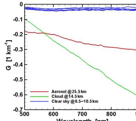
G (λ, z)=∂lnI (λ, z) /∂z, (1) where I (λ, z) is the limb radiance as a function of wave-lengthλand tangent heightz. The variation of the radiance gradient (i.e., the height derivative) with wavelength between 500 and 900 nm for various targets is shown in Fig. 1. Clear-sky scenes show Rayleigh scattering with almost no wave-length dependence, as expected. Note that the tropospheric cloud at 14.5 km shows a steeper wavelength dependence than the aerosol layer at 25.5 km. At visible and near-IR wavelengths longer thanλs=674 nm, where the absorption of light by ozone can be neglected, the dependence of the ra-diance gradient on wavelength can be parameterized using a linear relationship.

G (λ, z)≈α (z) (λ−λs)+k(z);λ≥λs, (2) whereαandk– the slope and intercept, respectively – are a function ofzand independent of wavelengthλ. Thus, the ab-solute value ofαis the measure of the strength of the spectral variation in radiance gradient. The slopeαin Eq. (2) can be

Figure 1. Variations in the radiance gradient G(λ, z) from OMPS/LP data at 5◦S during orbit 16754 on 21 January 2015. Blue: clear sky; green: cloud; red: aerosol.

determined by choosing a longer wavelength (λl):

α (z)=[G (λs, z)−G (λl, z)](λs−λl) . (3)

We choose the two wavelengths λs and λl within the LP measurement range to maximize the cloud signature. As the shorter wavelengthλs, 674 nm is chosen to avoid Chappuis band ozone absorption. Data rate limitations on the S-NPP spacecraft mean that not all possible wavelengths and alti-tudes measured by LP can be downloaded during regular op-erations. Although LP measurements extend to∼1015 nm, changes in spectral coverage during the S-NPP mission mean that 868 nm represents the longest wavelengthλl which is used in Eq. (3) available with full temporal coverage.

Calculating the slope values for the cases shown in Fig. 1, we find that α(6.5∼10.5 km)≈0 is consistent with the spectrally independent gradient expected for clear sky, α(25.5 km)= −0.00027 represents the weaker spec-tral dependence of radiance gradient for an aerosol, and

α(14.5 km)= −0.0013 corresponds to the strongest spectral dependence of radiance gradient for a cloud. We note that, since the slope values are typically negative, we can rewrite Eq. (3) to define the gradient difference ln R(z):

ln R(z)=[G (λs, z)−G (λl, z)]=α(z) (λs−λl) . (4)

(3)

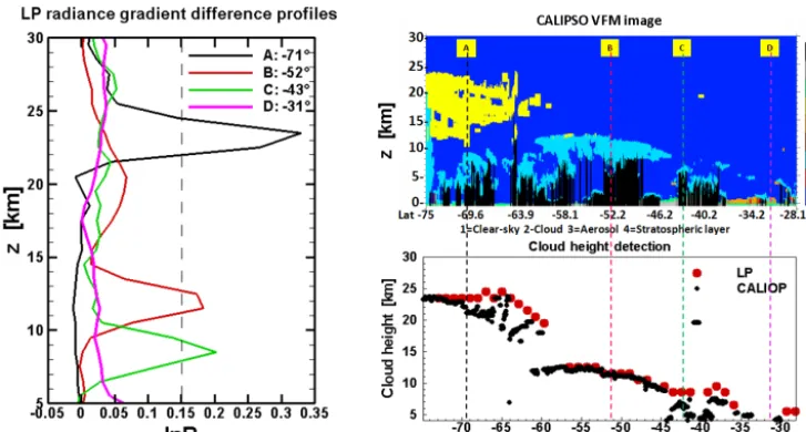
Figure 2. Radiance gradient and cloud detection results for four Southern Hemisphere events from a single orbit on 16 August 2012, using

OMPS/LP measurements and CALIPSO vertical feature mask (VFM) daytime data. Left panel: vertical profiles of the LP radiance gradient ln R for each event. The dashed black line represents the cloud detection threshold, which identifies clouds in events A, B, and C. Top right panel: CALIPSO VFM image for the same orbit. Yellow features indicate polar stratospheric clouds (PSCs), and light blue patches represent clouds. Bottom right panel: cloud height values detected by the LP algorithm (red dots) and from CALIPSO VFM data (black dots) in the same orbit. The four colored dotted lines in the right panel indicate the four events labeled as A, B, C, and D.

3 Results

3.1 Threshold determination

The method described in Sect. 2 has been used to determine cloud-top height from OMPS/LP measurements. We assign a positive cloud detection if the value of ln R in Eq. (2) meets a threshold value F at some altitude in the radiance gradient profile. To determine the cloud detection thresh-old, we use CALIPSO 532 nm backscattering daytime data (Winker et al., 2003) and the corresponding CALIPSO ver-tical feature mask (VFM) version 3 data product (Vaughan et al., 2004; Kacenelenbogen et al., 2011) on selected days where the satellite tracks of Suomi NPP and CALIPSO most closely overlap. Figure 2 provides an example of the deter-mination ofF during S-NPP orbit 4163 on 16 August 2012 for three events with clouds as well as one event without a cloud. These events show distinctly different signatures in their ln R profiles. The sharpest vertical gradient, with a maximum value of ln R=0.33 at 23.5 km, is observed for a polar stratospheric cloud (PSC). For clouds at lower al-titudes, the maximum values of ln R fall between 0.18 and 0.20. However, for the clear-sky event, the maximum value of ln R is very small (less than 0.05). Further comparisons with CALIPSO observations indicate thatF =0.15 is a rea-sonable threshold for positive cloud detection in LP data. 3.2 Influence of aerosols

Confirming the presence of a cloud at any altitude requires an ability to discriminate between cloud and aerosol signals.

We define a quantity called aerosol scattering index (ASI) at 674 nm for detecting aerosols in LP measurements:

ASI=_(I_m−Ic0) /Ic0, (5)

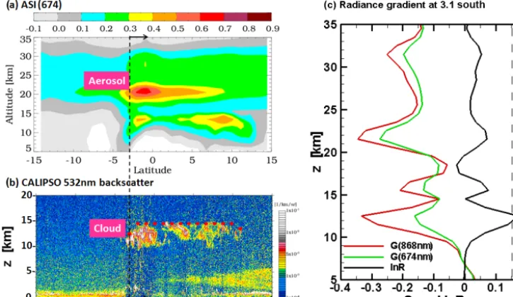
whereImis the measured radiance andIc0is the calculated radiance using a forward model (Herman et al., 1995) for a Rayleigh atmosphere. BothIm andIc0 are normalized at 45 km, assuming that there is no aerosol at that altitude. Figure 3a shows aerosols at 20–22 km at tropical latitudes, identified using ASI values for a single orbit on 19 June 2014. Although ASI is sensitive to stratospheric aerosols, ASI values also increase in the presence of clouds, so that this quantity alone does not distinguish between aerosols and clouds. Figure 3b shows clouds at 10–15 km identified by CALIPSO data for the same event. In the CALIPSO im-age, the red–gray–white colored features indicate clouds be-tween 10 and 15 km detected by lidar data, and the red dots represent LP cloud height values detected by our new algo-rithm for the same orbit. Note that the LP cloud locations are consistently at the top of the CALIPSO cloud regions. Figure 3c illustrates the LP radiance gradient profiles for a single event at 3◦_{S, identified by the dashed line in Fig. 3a}

(4)

Figure 3. Example of discrimination between clouds and aerosols, using OMPS/LP observations taken on 19 June 2014. (a) Aerosol layer at

20–22 km in tropics identified using OMPS/LP aerosol scattering index (ASI). (b) Tropospheric clouds at 10–15 km identified in CALIPSO data for the same orbit. The red dots represent LP cloud-top height values derived from the radiance gradient algorithm. (c) LP radiance gradient profiles (red: 868 nm; green: 674 nm) for a single event at 3.1◦S, identified by the dashed line in panels (a) and (b). The difference between profiles (ln R) is shown as the black line.

Figure 4. ln R (solid line) and ASI (dashed line) plotted as a function of single-scattering angle (SSA) at 14.5 km (green) and 20.5 km (red).

This figure uses OMPS/LP observations taken on 19 June 2014, from the same orbit shown in Fig. 3. The dotted black line represents the value of the cloud detection threshold for the ln R curves.

The OMPS/LP viewing geometry produces high single-scattering angle (SSA) values for Southern Hemisphere mea-surements (up to 160◦) and low SSA values for Northern Hemisphere measurements (down to 20◦). This relationship leads to large variations in ASI values over an orbit due to Mie scattering phase function effects. Figure 4 shows the variation of ln R and ASI as a function of SSA at 14.5 and 20.5 km for the same orbit presented in Fig. 3. ASI values increase rapidly for SSA<80◦at both altitudes. In contrast, ln R values are essentially constant throughout the orbit and are well below our cloud detection threshold except for the tropical region that is consistent with CALIPSO cloud

detec-tions. We therefore use a constant cloud detection threshold to evaluate all LP measurements.

3.3 Comparison with LP Version 2 results

(5)

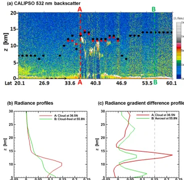
Figure 5. Comparison of LP cloud detection results for a single orbit on 16 August 2012. (a) CALIPSO 532 nm daytime backscatter

data for the same orbit. The red–gray–white regions in the image denote the cloud layers. The red and black dots in the image represent cloud-top heights derived from the LP radiance gradient algorithm and the LP Version 2 algorithm, respectively. Lines A and B indicate OMPS/LP measurements at 36.5 and 55.8◦N, respectively. (b) Radiance profiles at 892 nm used as the basis for LP Version 2 algorithm cloud identification. Red: event A; green: event B. (c) Radiance gradient difference profiles used for new LP algorithm cloud identification. Red: event A; green: event B. The dashed line represents the value of the cloud detection threshold.

2012, with comparisons to the CALIPSO 532 nm backscat-ter coefficient for the same orbit. The LP Version 2 algo-rithm identifies many clouds that are not seen by CALIPSO, while the radiance gradient method only finds a few higher clouds between 33 and 46◦_{N at locations where CALIPSO}

also shows such clouds. This suggests that the LP Version 2 algorithm may misidentify aerosols as clouds. To further il-lustrate this result, we focus on two selected events at 36.5◦N (event A) and 55.8◦N (event B). The LP Version 2 algorithm finds sufficiently sharp changes in 892 nm radiance profiles to identify clouds at 14.5 km for both events (Fig. 5b). In contrast, the radiance gradient algorithm finds a clear cloud signature in ln R values for event A, but a much weaker sig-nature that falls below the detection threshold for event B (Fig. 5c). These results give us confidence that the radiance gradient algorithm is not creating “false-positive” cloud

iden-tifications. Removing the incorrect cloud detections will also provide increased sampling in the upper troposphere for LP retrieval products.

4 Validation of LP cloud height product

In order to quantify the accuracy of LP cloud-top height values derived by the new LP radiance gradient algo-rithm, we evaluate our results against the CALIPSO VFM daytime product. The similarity in orbits between the S-NPP and CALIPSO spacecraft makes it possible to se-lect many events with reasonably tight coincidence cri-teria (1latitude<±0.15◦, 1longitude<±3.25◦, 1time<

(6)

re-1244 Z. Chen et al.: A new algorithm for detecting cloud height

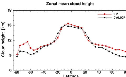
Figure 6. Zonal mean cloud height calculated from LP cloud

de-tection algorithm results (red line) and collocated CALIPSO data (black line) in 5◦latitude bands. Results averaged over 70 sample days between April 2012 and February 2015.

quirements yielded approximately 439 000 cases spread over 70 sample days between April 2012 and February 2015. We do not consider LP cloud detections below 5 km because our approach is not effective at such low altitudes.

Figure 6 shows the latitude distribution of cloud-top heights from these coincidence data sets in 5◦zonal mean lat-itude bands. The cloud-top heights derived from the LP algo-rithm agree quite well with CALIPSO data in the tropics and midlatitudes (up to approximately 50◦). The cloud altitudes derived from both data sets decrease towards the poles due to the general decrease of the tropopause height. The LP cloud height values are higher in polar regions because our data set consistently includes PSCs, which are identified at 15–30 km in winter and spring months (see example in Fig. 2). LP mea-surements may also detect clouds that are located at different positions along the line of sight, which would give lower de-rived cloud heights than if the same cloud were located at the tangent point position.

Figure 7 shows a histogram of cloud height differences be-tween the LP and CALIPSO data sets. The difference values are calculated as the LP cloud-top height minus the collo-cated CALIPSO value. The histogram has been constructed using bins of 1 km, the vertical sampling of the LP mea-surements. The most common difference values occur be-tween−1 and+4 km, with a median difference of1zcloud= 1.8 km. A Gaussian fit to these data yields a similar median difference value (2.0 km). We note that the LP cloud detec-tion algorithm identifies the upper edge of a cloud, so it is not surprising to find a high bias in reported heights relative to CALIPSO cloud height values based on nadir-viewing li-dar measurements. In addition, the LP vertical resolution is ∼1.6–1.8 km, whereas CALIPSO data have much finer ver-tical sampling and resolution. The extended tail of this distri-bution towards large negative values corresponds to scattered high-cloud values (zcloud>20 km) in the CALIPSO data set.

-15 -10 -5 0 5 10 15

Difference (LP–CALIOP) [km]

0.00 0.02 0.04 0.06 0.08 0.10

Normalized frequency

Mean fit=2.0

Median=1.8 Sigma=4.9

Figure 7. Normalized frequency histogram of all cloud height

dif-ferences (LP−CALIPSO) from coincidence data sets in1zcloud= 1 km intervals. The red curve represents a Gaussian fit to the data.

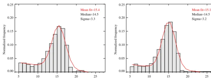
Figure 8 shows two histograms of cloud-top heights in the tropics as detected from the LP algorithm and from CALIPSO data. These distributions have very similar shapes, and the distributions are roughly Gaussian. The maximum cloud height occurrence frequency is observed between 14 and 16 km for both instruments. We note that the CALIPSO data show some clouds up to 25 km height, which confirms previous studies that CALIPSO can sometimes misidentify aerosols as clouds (Chen et al., 2010, 2012). However, the LP data set does identify a population of clouds at 20–22 km, which are clearly above the tropopause when individual or-bits are inspected. The presence of these unusually high clouds in the tropics is connected with Kelut Volcano, which erupted in February 2014. Remember that the ln R value cal-culation presented in Sect. 2 determines the slope of the ra-diance gradient. Larger aerosol particles, such as those found in fresh volcanic plumes, will increase the slope of the radi-ance gradient and makes these events more difficult to dis-tinguish from “normal” clouds. In addition, patchy clouds in the near and far sides of the tangent point may also cause biased estimates of cloud height. This potential error source was investigated in detail by Kent et al. (1997).

5 Summary and conclusions

(7)

consis-5 10 15 20 25 LP_CloudHeight [km] 0.00 0.05 0.10 0.15 0.20 0.25 Normalized frequency Mean fit=15.4 Median=14.5 Sigma=3.3

5 10 15 20 25

CALIOP_CloudHeight [km] 0.00 0.05 0.10 0.15 0.20 0.25 Normalized frequency Mean fit=15.1 Median=14.5 Sigma=3.2

Figure 8. Normalized frequency histograms of all cloud height values from LP cloud detection results (left panel) and the collocated

CALIPSO data (right panel) in the tropics (latitude<±30◦) in1zcloud=1 km intervals. The red curves represent a linear combination of a Gaussian and quadratic function fit to each data set.

tent with CALIPSO observations in terms of latitude depen-dence and frequency distribution of altitudes. The offset in absolute cloud height for coincident measurements is consis-tent with differences between the detection methods. The LP cloud detection algorithm also consistently identifies polar stratospheric clouds in both hemispheres, which may be use-ful for directly examining the impact of PSCs on LP ozone retrievals. We do not attempt to retrieve cloud heights below 5 km with this algorithm. Aerosol layers with larger particles, such as fresh volcanic plumes, are more likely to be classi-fied as clouds. Further theoretical studies of spectral proper-ties and scattering effects are needed to fully understand the applicability range and limitations of this method. The new cloud detection algorithm will be implemented for the forth-coming LP Version 3 ozone and aerosol retrieval algorithms, and the LP cloud height values will also be distributed as a public data product.

Data availability

The OMPS/LP Level 1 gridded radiance product (LP-L1G-EV) used to create the cloud height product described in this paper can be obtained at https://ozoneaq.gsfc.nasa.gov/data/ ozone/, 2016.

Acknowledgements. We thank Mark Schoeberl for his

insight-ful comments on the development of this algorithm. Zhong Chen and Matthew DeLand were supported by NASA contract NNG12HP08C.

Edited by: D. Loyola

References

Bourassa A. E., Degenstein, D. A., and Llewellyn E. J.: Climatology of the subvisual cirrus clouds as seen by OSIRIS on Odin, Adv. Space Res., 36, 807–812, 2005.

Chen, B., Huang, J., Minnis, P., Hu, Y., Yi, Y., Liu, Z., Zhang, D., and Wang, X.: Detection of dust aerosol by combining CALIPSO active lidar and passive IIR measurements, Atmos. Chem. Phys., 10, 4241–4251, doi:10.5194/acp-10-4241-2010, 2010.

Chen, Z., Torres, O., McCormick, M. P., Smith, W., and Ahn, C.: Comparative study of aerosol and cloud detected by CALIPSO and OMI, Atmos. Environ., 51, 187–195, 2012.

Eichmann, K.-U., Lelli, L., von Savigny, C., Sembhi, H., and Bur-rows, J. P.: Global cloud top height retrieval using SCIAMACHY limb spectra: model studies and first results, Atmos. Meas. Tech., 9, 793–815, doi:10.5194/amt-9-793-2016, 2016.

Flynn, L. E., Seftor, C. J., Larsen, J. C., and Xu, P.: The Ozone Map-ping and Profiler Suite, in: Earth Science Satellite Remote Sens-ing, edited by: Qu, J. J., Gao, W., Kafatos, M., Murphy, R. E., and Salomonson, V. V., Springer, Berlin, 279–296, doi:10.1007/978-3-540-37293-6, 2007.

Herman, B. M., Caudill, T. R., Flittner, D. E., Thome, K. J., and Ben-David, A.: Comparison of the Gauss-Seidel spherical polar-ized radiative transfer code with other radiative transfer codes, Appl. Optics, 34, 4563–4572, 1995.

Jaross, G., Bhartia, P. K., Chen, G., Kowitt, M., Haken, M., Chen, Z., Xu, P., Warner, J., and Kelly, T.: OMPS Limb Profiler instru-ment performance assessinstru-ment, J. Geophys. Res.-Atmos., 119, 4399–4412, doi:10.1002/2013JD020482, 2014.

Kacenelenbogen, M., Vaughan, M. A., Redemann, J., Hoff, R. M., Rogers, R. R., Ferrare, R. A., Russell, P. B., Hostetler, C. A., Hair, J. W., and Holben, B. N.: An accuracy assessment of the CALIOP/CALIPSO version 2/version 3 daytime aerosol extinction product based on a detailed sensor, multi-platform case study, Atmos. Chem. Phys., 11, 3981–4000, doi:10.5194/acp-11-3981-2011, 2011.

Kent, G. S., Winker, D. M., Vaughan, M. A., Wang, P.-H., and Skeens, K. M.: Simulation of Stratospheric Aerosol and Gas Experiment (SAGE) II cloud measurements using airborne lidar data, J. Geophys. Res., 102, 21795–21807, doi:10.1029/97JD01390, 1997.

(8)

Kokhanovsky, A. A., Rozanov, V. V., Burrows, J. P., Eichmann, K. U., Lotz, W., and Vountas, M.: The SCIAMACHY cloud prod-ucts: Algorithms and examples from ENVISAT, Adv. Space Res., 36, 789–799, doi:10.1016/j.asr.2005.03.026, 2005.

Kuze, A. and Chance, K. V.: Analysis of cloud top height and cloud coverage from satellites using the O2A and B bands, J. Geophys. Res., 99, 14481–14491, 1994.

Loyola, D., Thomas, W., Livschitz, Y., Ruppert, T., Albert, P., and Hollmann, R.: Cloud properties derived from GOME/ERS-2 backscatter data for trace gas retrieval, IEEE T. Geosci. Remote, 45, 2747–2758, 2007.

Loyola, D., Thomas, W., Spurr, R., and Mayer, B.: Global pat-terns in daytime cloud properties derived from GOME backscat-ter UV-VIS measurements, Int. J. Remote Sens., 31, 4295–4318, 2010.

OMPS/LP Level 1: OMPS Limb Profiler Suomi NPP-LP-L1G-EV, available at: https://ozoneaq.gsfc.nasa.gov/data/ozone/, last ac-cess: 22 March 2016.

Rault, D. F. and Loughman, R. P.: The OMPS Limb Profiler Envi-ronmental Data Record algorithm theoretical basis document and expected performance, IEEE T. Geosci. Remote, 51, 2505–2527, 2013.

Rozanov, V. V. and Kokhanovsky, A. A.: Semianalytical cloud re-trieval algorithm as applied to the cloud top altitude and the cloud geometrical thickness determination from top-of-atmosphere re-flectance measurements in the oxygen A band, J. Geophys. Res., 109, D05202, doi:10.1029/2003JD004104, 2004.

Schuessler, O., Loyola, D., Doicu, A., and Spurr, R.: Information Content in the Oxygen A-Band for the Retrieval of Macrophysi-cal Cloud Parameters, IEEE T. Geosci. Remote, 52, 3246–3255, 2014.

van Diedenhoven, B., Hasekamp, O. P., and Landgraf, J.: Retrieval of cloud parameters from satellite-based reflectance measure-ments in the ultraviolet and the oxygen A-band, J. Geophys. Res., 112, D15208, doi:10.1029/2006JD008155, 2007.

Vaughan, M., Young, S., Winker, D., Powell, K., Omar, A., Liu, Z., Hu, Y., and Hostetler, C.: Fully automated analysis of spacebased lidar data: an overview of the CALIPSO retrieval algorithms and data products, Proc. SPIE, 5575, 16–30, 2004.

von Savigny, C., Ulasi, E. P., Eichmann, K.-U., Bovensmann, H., and Burrows, J. P.: Detection and mapping of polar stratospheric clouds using limb scattering observations, Atmos. Chem. Phys., 5, 3071–3079, doi:10.5194/acp-5-3071-2005, 2005.