www.ocean-sci.net/6/633/2010/ doi:10.5194/os-6-633-2010
© Author(s) 2010. CC Attribution 3.0 License.
Ocean Science
Numerical implementation and oceanographic application of the
thermodynamic potentials of liquid water, water vapour, ice,
seawater and humid air – Part 1: Background and equations
R. Feistel1, D. G. Wright2,†, D. R. Jackett3, K. Miyagawa4, J. H. Reissmann5, W. Wagner6, U. Overhoff6, C. Guder6, A. Feistel7, and G. M. Marion8
1Leibniz-Institut f¨ur Ostseeforschung, Seestraße 15, 18119 Warnem¨unde, Germany 2Bedford Institute of Oceanography, Dartmouth, NS, B2Y 4A2, Canada
3CSIRO Marine and Atmospheric Research, P.O. Box 1538, Hobart, TAS 7001, Australia 44-12-11-628, Nishiogu, Arakawa-ku, Tokyo, 116-0011, Japan
5Bundesamt f¨ur Seeschifffahrt und Hydrographie, Bernhard-Nocht-Straße 78, 20359 Hamburg, Germany 6Ruhr-Universit¨at Bochum, Lehrstuhl f¨ur Thermodynamik, 44780 Bochum, Germany
7Technische Universit¨at Berlin, Einsteinufer 25, 10587 Berlin, Germany 8Desert Research Institute, Reno, NV, USA
†Dan Wright tragically passed away in July 2010
Received: 24 November 2009 – Published in Ocean Sci. Discuss.: 15 March 2010 Revised: 29 June 2010 – Accepted: 29 June 2010 – Published: 14 July 2010
Abstract. A new seawater standard referred to as the Interna-tional Thermodynamic Equation of Seawater 2010 (TEOS-10) was adopted in June 2009 by UNESCO/IOC on its 25th General Assembly in Paris, as recommended by the SCOR/IAPSO Working Group 127 (WG127) on Thermody-namics and Equation of State of Seawater. To support the adoption process, WG127 has developed a comprehensive source code library for the thermodynamic properties of liq-uid water, water vapour, ice, seawater and humid air, referred to as the Sea-Ice-Air (SIA) library. Here we present the back-ground information and equations required for the determi-nation of the properties of single phases and components as well as of phase transitions and composite systems as im-plemented in the library. All results are based on rigorous mathematical methods applied to the Primary Standards of the constituents, formulated as empirical thermodynamic po-tential functions and, except for humid air, endorsed as Re-leases of the International Association for the Properties of Water and Steam (IAPWS). Details of the implementation in the TEOS-10 SIA library are given in a companion paper.
Correspondence to: R. Feistel
1 Introduction
The recent availability of highly accurate mathematical for-mulations of thermodynamic potentials for fluid water (Wag-ner and Pruß, 2002; IAPWS, 2009a), air (Lemmon et al., 2000; Feistel et al., 2010a), ice (Feistel and Wagner, 2006; IAPWS, 2009b), and of seawater (Feistel, 2003, 2008; Millero et al., 2008; IAPWS, 2008a; IOC et al., 2010) permit the description of thermodynamic properties of the ocean and the atmosphere in an unprecedented comprehen-sive and consistent manner (Feistel et al., 2008; IOC et al., 2010). In June 2009 these formulations, jointly referred to as the International Thermodynamic Equation of Seawa-ter 2010 (TEOS-10), were adopted by UNESCO/IOC as the successor of the International Equation of State of Seawa-ter 1980 (EOS-80). To assist potential users in implement-ing the new equations of state, the SCOR1/IAPSO2 Work-ing Group 127 (WG127) on Thermodynamics and Equa-tion of State of Seawater has developed a source code li-brary in Fortran and Visual Basic (also for use with Excel) which provides an extended set of functions for the compu-tation of numerous properties of the geophysical fluids, their composites and phase transitions. Equivalent versions of the SIA library implemented in MatLab and C/C++ are planned.
1SCOR: Scientific Committee on Oceanic Research,
http://www.scor-int.org
2IAPSO: International Association for the Physical Sciences of
Additional library versions are available for specific applica-tion purposes such as the Gibbs SeaWater (GSW) Library for oceanographic models (IOC et al., 2010), consistent with the one described in this paper. This SIA library replaces (i.e., updates and extends) the code versions published previously (Feistel, 2005; Feistel et al., 2005).
In this paper we provide formulas, derivations and expla-nations for the quantities implemented in the library and their thermodynamic relations to the potential functions. The lat-ter are basic relations which remain valid independent of any details of the fits used to approximate the potentials or the numerics used to evaluate the functional relations; they will not change when new approximations to the thermodynamic potentials are determined in the future.
The oceanographic applications of the quantities discussed here are explained in detail in IOC et al. (2010). Formulas for seawater properties at the ocean-atmosphere interface such as the vapour pressure and the latent heat in equilibrium with humid air consistent with the library functions described here are developed in a separate article (Feistel et al., 2010a). Ad-ditional details on the library structure and the numerical im-plementation are available from a companion paper (Wright et al., 2010a).
The code is organised in vertical columns representing the four constituents: fluid water, ice, seawater and air, and in horizontal levels with increasing complexity at higher lev-els. The code is hierarchically organised; higher level rou-tines make use of rourou-tines from lower levels but code at each level neither needs nor has access to procedures from higher levels. Level 0 provides fundamental constants, mathemat-ical methods and formulae for conversions between Abso-lute Salinity and Practical Salinity given the measurement location plus some general relations. Level 1 contains the Primary Standards, i.e. the thermodynamic potentials, their basic constants and coefficients, and further necessary em-pirical or theoretical functions. Levels 2–4 contain proper-ties derived directly or indirectly from level 1 by mathemat-ical and numermathemat-ical manipulations without additional empiri-cal formulas or constants. Level 2 contains explicit relations. Levels 3 and 4 require iteration procedures to numerically solve implicit equations. Levels 1–3 describe only single-phase properties, while level 4 procedures calculate single-phase equilibria and properties of composite, multi-phase systems. Level 5 is an additional application layer within which input and output units may be more convenient for the user than the basic SI units that are used rigorously at the lower lev-els. Level 5 also contains additional empirical coefficients in speed-optimized code, derived as “approximate” correlation functions representing reduced data sets computed from the lower, “exact” levels.
The following sections explain the thermodynamic rela-tions and auxiliary equarela-tions implemented in the library level by level, with the exception of level 0, which provides gen-eral information required by the library, and level 5, which is only numerically different from the lower ones. Within each
level, the sections consider the four columns or their combi-nations. In the appendix, the formulas are described which are implemented in the library to iteratively solve implicit equations. When appropriate, function names defined in the library are mentioned in the text of this paper along with the related equations; they are emphasized by means of a distinct
font type. The complete list of modules and functions
avail-able from the library is described in the companion paper, Part 2 (Wright et al., 2010a).
The core levels 1–4 of the SIA library take as input pa-rameters absolute pressure in Pa, absolute ITS-90 tempera-ture in K, and Absolute Salinity in kg/kg. Absolute Salin-ity of Standard Seawater is most accurately estimated by Reference Salinity (Millero et al., 2008) which is propor-tional to Practical Salinity in the valid range of the 1978 Practical Salinity Scale (PSS-78). For seawater with com-position anomalies, estimates for the difference between Ab-solute and Reference Salinity are available for the global ocean and the Baltic Sea (McDougall et al., 2009; IOC et al., 2010; Feistel et al., 2010b). A routine for conversions between Practical Salinity and Absolute Salinity is included in the SIA library at level 0 (functionsasal from psal
and psal from asal) using an algorithm adapted from
the GSW library (McDougall et al., 2009). A function that permits the computation of Density Salinity as an es-timate of Absolute Salinity from measured in situ density, e.g., in the laboratory, is also available in the SIA library (function sea sa si). Further details are available from the companion paper, Part 2 (Wright et al., 2010a). De-tails on the use and the uncertainties of the different salin-ity scales are described by Wright et al. (2010b). Con-version routines between different pressure units (function
cnv pressure), temperature scales and units (function
cnv temperature), as well as between various salinity measures (functioncnv salinity) are available at level 5 of the library for convenience.
In order to shorten the main article for technical reasons, 29 tables with groups of thermodynamic properties and their equations were moved to the Digital Supplement of this pa-per. They are referred to here as Table S1 to S29; their equa-tions are numbered as S1.1 etc. Because of their key role in the SIA library, the various potential functions themselves are summarised in Table 1 rather than in the supplement.
Table 1. Hierarchy of thermodynamic potentials and their elementary constituents implemented in the library.
Potential Level Routine Parent System Reference
fF(T , ρ) 1 flu f si Primary Fluid water Sect. 2.1 gIh(T , P ) 1 ice g si Primary Ice Ih Sect. 2.2 gi(T , P ) 1 sal g term si Primary Seawater Eq. (2.2)
fA(T , ρ) 1 dry f si Primary Dry Air Eq. (2.6) BAW(T ) 1 air baw m3mol Primary Humid Air Sect. 2.4
CAWW(T ) 1 air caww m6mol2 Primary Humid Air Sect. 2.4
CAAW(T ) 1 air caaw m6mol2 Primary Humid Air Sect. 2.4
gS(SA, T , P ) 2 sal g si gi Seawater Eq. (2.2)
fmix(A, T , ρ) 2 air f mix si BAW, Humid Air Eq. (2.13)
CAWW,
CAAW
fAV(A, T , ρ) 2 air f si fF,fA,fmix Humid Air Eq. (2.7) gW(T , P ) 3 liq g si fF Liquid water Eq. (4.2) gV(T , P ) 3 vap g si fF Water vapour Eq. (4.3) gSW(SA, T , P ) 3 sea g si gW,gS Seawater Eq. (4.4)
hSW(SA, η, P ) 3 sea h si gSW Seawater Eq. (4.5)
gAV(A, T , P ) 3 air g si fAV Humid Air Eq. (4.37) hAV(A, η, P ) 3 air h si gAV Humid Air Eq. (4.40) gSI(SSI, T , P ) 4 sea ice g si gSW,gIh Seawater + Eq. (5.14)
ice
gSV(SSV, T , P ) 4 sea vap g si gSW,gV Seawater Eq. (5.30)
+ water vapour
gAW(wA, T , P ) 4 liq air g si gW,gAV Liquid water Eq. (5.58)
+ humid air
hAW(wA, η, P ) 4 liq air h si gAW Liquid water Eq. (5.63)
+ humid air
gAI(wA, T , P ) 4 ice air g si gIh,gAV Ice Eq. (5.73)
+ humid air
hAI(wA, η, P ) 4 ice air h si gAI Ice Eq. (5.78)
+ humid air
gW F03(T , P ) 5 fit liq g f03 si Fit offF Liquid water IAPWS (2009c)
gW IF97(T , P ) 5 fit liq g if97 si Fit offF Liquid water IAPWS (2007)
gV IF97(T , P ) 5 fit vap g if97 si Fit offF Water vapour IAPWS (2007)
library decided that the published molar equation can be con-verted to the mass-based form used here and in the planned IAPWS document (IAPWS, 2010), and that this should be implemented using the latest value for the molar mass of dry air (Picard et al., 2008) rather than the originally published one. For consistency with the IAPWS formulation, the molar mass of dry air of the SIA library is updated in the SIA ver-sion 1.1, attached as a supplement to the companion paper (Wright et al., 2010a), in contrast to the obsolete value used in SIA version 1.0 which is consistent with the formulation of Feistel et al. (2010a).
2 Level 1: Thermodynamic potentials – the primary standard
As described in the related background articles, the vast amount of quantitative information available from extensive sets of experimental thermodynamic data for water, ice, sea-water and air is represented in a compact way by the em-pirical coefficients of only four independent functions, a Helmholtz function fF(T ,ρ) of fluid water referred to as IAPWS-95 (IAPWS, 2009a; Wagner and Pruß, 2002), a Gibbs function gIh(T ,P ) of ice, referred to as IAPWS-06 (IAPWS, 2009b; Feistel and Wagner, 2006), a Gibbs func-tiongS(SA,T ,P )of sea salt dissolved in water which is
-14 -13 -12 -11 -10 -9 -8 -7 -6 -5 -4 -3 -2 -1 0 1 2 3 4100 200 300 400 500 600 700 800 900 1000 1100 1200 1300 T em pe ra tur e T /K
Density lg(ρ/(kg m-3 ) )
a) Density - Temperature Diagram of Liquid Water and Vapour
CP CP CP CP TP TP TP
TP TPTPTPTP
Liquid LiquidLiquid Liquid + ++ + Vapour Vapour Vapour Vapour 130 K 130 K130 K 130 K 1000 °C 1000 °C 1000 °C 1000 °C 0 °C 0 °C 0 °C 0 °C
Sublimation Line Sublimation Line Sublimation Line Sublimation Line Ice IhIce IhIce IhIce Ih
Vapou r Vapou r Vapou r Vapou r 10 nP a 10 n Pa 10 nP a 10 n P a 10 0 P a 10 0 P a 10 0 P a 10 0 P a 10 1 3 25 P a 10 1 3 25 P a 10 1 3 25 P a 10 1 3 25 P a 10 M P a 10 M P a 10 M P a 10 M P a 10 0 M P a 10 0 M P a 10 0 M P a 10 0 M P a 1 G P a 1 G P a 1 G P a 1 G P a Ice Ice Ice Ice
950 1000 1050 1100 1150 1200 1250
250 260 270 280 290 300 310 320 330 340 350 360 T em pe ra tur e T /K
Density ρ/(kg m -3 )
b) Density - Temperature Diagram of Liquid Water
TP TPTP TP 2 Phases 2 Phases2 Phases 2 Phases 0 °C 0 °C 0 °C 0 °C 40 °C 40 °C 40 °C 40 °C Liquid Water Liquid Water Liquid Water Liquid Water N ep tu nian N eptu nian N eptu nian N ep tu nian R an ge R an ge R an ge R an ge Freezin g Point Freezing Point Freezing Point Freezin g Point Lowering Lowering Lowering Lowering V ap ou r P re ssur
e Lin e V ap ou r P re ss ur e Lin
e V ap ou r P re ss ur
e Lin e V ap ou r P re ssur
e Lin e 10 1 3 25 P a 10 1 3 25 P
a 10
1 3 25 P
a 10 1 3 25 P a 10 0 M P a 10 0 M Pa 10 0 M Pa 10 0 M P a 1 G P a 1 G P a 1 G P a 1 G P a Ice Ih Ice Ih Ice Ih Ice Ih Ice III Ice III Ice III Ice III
Ice V Ice V Ice V Ice V
Ice V I Ice V I Ice V I Ice V I
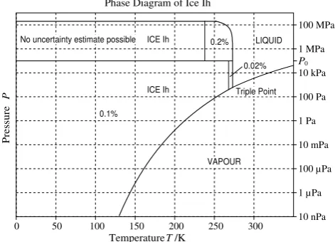
Fig. 1. Panel (a) Validity region (bounded by bold lines) of the
IAPWS-95 Helmholtz potential for fluid water with isobars as indi-cated. Panel (b) Magnified view of the small region corresponding to the standard oceanographic (“Neptunian”) range. TP: triple point gas-liquid-solid, CP: critical point. The deviation of the vapour-pressure line from the 101 325 Pa isobar in the liquid region is be-low the graphical resolution of panel (b). Freezing-point be-lowering occurs with the addition of sea salt. To deal with this effect in the case of seawater, the extension of the pure water properties into the metastable liquid region just above the line marked “Freezing Point Lowering” is required.
al., 2000) in combination with air-water cross-virial coeffi-cients (Hyland and Wexler, 1983; Harvey and Huang, 2007; Feistel et al., 2010a). These potential functions are used as the Primary Standard for pure water (liquid, vapour and solid), seawater and humid air from which all other proper-ties are derived by mathematical operations, i.e. without the need for additional empirical functions.
0 50 100 150 200 250 300 10 nPa
1 µPa 100 µPa 10 mPa 1 Pa 100 Pa 10 kPa 1 MPa 100 MPa P re ss ur e P
Temperature T /K
Phase Diagram of Ice Ih
P0 Triple Point LIQUID VAPOUR ICE Ih ICE Ih No uncertainty estimate possible
0.1%
0.02% 0.2%
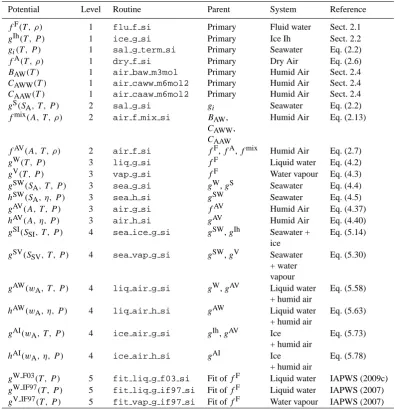
Fig. 2: Range of validity (bold curves) of the Gibbs function of ice Ih and uncertainty of density.
2.3Sea Salt Dissolved in Water
The Gibbs function gSW(SA,T,P) of seawater (IAPWS, 2008a; Feistel, 2008) is expressed as
the sum of a Gibbs function for pure water, gW(T,P), numerically available from the
IAPWS-95 formulation, and a saline part, g(SA,T,P)
S :
(S T P) g (TP) g(S TP)
g , , , A, ,
S W A
SW = + . (2.1)
Here, salinity is expressed as Absolute Salinity SA, the mass fraction of dissolved salt in
seawater, which for standard seawater equals the Reference-Composition Salinity within experimental uncertainty (Millero et al., 2008; Wright et al., 2010b).
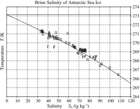
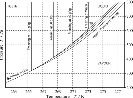
In representing the properties of Standard Seawater, the range of validity of the Gibbs function for seawater is shown in Fig. 3. For temperatures in the oceanographic standard range, salinities up to 40 g/kg are properly described up to 100 MPa. For higher salinities up to 120 g/kg and temperatures up to 80 °C, the application is restricted to atmospheric pressure (101 325 Pa). Up to saturation, the salinity of cold concentrated brines agrees well with Antarctic sea-ice data (Fig. 6). For hot concentrates (region F in Fig. 3) the partial derivatives of density are not reliable. New density measurements (Millero and Huang, 2009; Safarov et al., 2009) have led to some recent improvements and an option to use an extension introduced Fig. 2. Range of validity (bold curves) of the Gibbs function of ice
Ih and uncertainty of density.
2.1 Fluid water
The validity range of the IAPWS-95 Helmholtz potential fF(T ,ρ)for fluid water (IAPWS, 2009a; Wagner and Pruß, 2002) as a function of temperatureT and densityρis shown in Fig. 1a in a density-temperature diagram. It is confined to the pressure interval between the isobars of 10 nPa and 1 GPa, below the upper temperature bound of 1000◦C and by the phase transition lines with ice and the liquid-vapour 2-phase region. Below the critical temperature, this region separates the stable vapour phase at low density from the sta-ble liquid phase at high density. Only a small fraction of this region (a subset of the sliver to the right of the high density side of the phase transition boundary) belongs to the “Nep-tunian” oceanographic standard range (Fig. 1b). In the pres-ence of dissolved sea salt, the freezing point is lowered so that the liquid phase of water is extended into the ice and vapour regions indicated in Fig. 1b.
The Helmholtz function fF(T ,ρ) together with its first and second partial derivatives is implemented as the library functionflu f si.
2.2 Ice
R. Feistel et al.: Oceanographic application and numerical implementation of TEOS-10: Part 1 637
by Feistel (2010) is included in the library (Wright et al., 2010a). Nevertheless, reliability of results for this region remains limited by the sparseness of data and the possibility of precipitation of calcium minerals (Marion et al., 2009) which would degrade the accuracy of the Reference Composition approximation in this region.
SA / (g kg-1)
t / °C lg(P /P0 )
0 -20
20 40
60
80
20
40
60
80
100
120
140 1
2 3
-1
-2
-3
Fre ezin
g S
urfac e
Sublim
ation
Line Triple
Lin e
Vap our-Pressure
Surface TP
ICE
VAPOUR
LIQUID WATER
A
B
C D
E
F 0.002%
0.001% 0.0004%
0.02
% 0.
2% 1%
3%
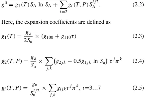
Fig. 3 Range of validity of the IAPWS-08 Gibbs function of seawater and uncertainty of density estimates calculated from this function. Region A: oceanographic standard range, B: extension to higher salinities, C: hot concentrates, D: zero-salinity limit, E: extrapolation into the metastable region below 0 °C.
The saline part g(SA,T,P)
S of the Gibbs function together with its first and second partial
derivatives is implemented as the library function sal_g_si.
Note that the arguments of the Gibbs function are temperature and pressure rather than temperature and density as in the Helmholtz function. Since the Gibbs function of pure water
is expressed in terms of the corresponding Helmholtz function, sea_g_si is only available at
library level 3 where implicitly determined quantities, such as density in terms of temperature and pressure, are considered.
Fig. 3. Range of validity of the IAPWS-08 Gibbs function of
seawa-ter and uncertainty of density estimates calculated from this func-tion. Region A: oceanographic standard range, B: extension to higher salinities, C: hot concentrates, D: zero-salinity limit, E: ex-trapolation into the metastable region below 0◦C.
the vapour equation down to 50 K is implemented that per-mits the computation of sublimation properties to this limit (IAPWS, 2008c; Feistel et al., 2010a). Vapour cannot rea-sonably be expected to exist below 50 K (Feistel and Wag-ner, 2007). No ice forms other than Ih occur naturally under oceanographic conditions.
The Gibbs functiongIh(T ,P )together with its first and second partial derivatives is implemented as the library func-tionice g si.
2.3 Sea salt dissolved in water
The Gibbs function gSW(SA,T ,P ) of seawater (IAPWS,
2008a; Feistel, 2008) is expressed as the sum of a Gibbs function for pure water, gW(T ,P ), numerically avail-able from the IAPWS-95 formulation, and a saline part, gS(SA,T ,P ):
gSW(SA,T ,P )=gW(T ,P )+gS(SA,T ,P ). (2.1)
Here, salinity is expressed as Absolute SalinitySA, the mass
fraction of dissolved salt in seawater, which for standard sea-water equals the Reference-Composition Salinity within ex-perimental uncertainty (Millero et al., 2008; Wright et al., 2010b).
In representing the properties of Standard Seawater, the range of validity of the Gibbs function for seawater is shown in Fig. 3. For temperatures in the oceanographic standard range, salinities up to 40 g/kg are properly described up to 100 MPa. For higher salinities up to 120 g/kg and tempera-tures up to 80◦C, the application is restricted to atmospheric
pressure (101 325 Pa). Up to saturation, the salinity of cold concentrated brines agrees well with Antarctic sea-ice data (Fig. 6). For hot concentrates (region F in Fig. 3) the partial derivatives of density are not reliable. New density measure-ments (Millero and Huang, 2009; Safarov et al., 2009) have led to some recent improvements and an option to use an ex-tension introduced by Feistel (2010) is included in the library (Wright et al., 2010a). Nevertheless, reliability of results for this region remains limited by the sparseness of data and the possibility of precipitation of calcium minerals (Marion et al., 2009) which would degrade the accuracy of the Refer-ence Composition approximation in this region.
The saline part gS(SA,T ,P ) of the Gibbs function
to-gether with its first and second partial derivatives is imple-mented as the library functionsal g si.
Note that the arguments of the Gibbs function are temper-ature and pressure rather than tempertemper-ature and density as in the Helmholtz function. Since the Gibbs function of pure water is expressed in terms of the corresponding Helmholtz function,sea g siis only available at library level 3 where implicitly determined quantities, such as density in terms of temperature and pressure, are considered.
The functiongS(SA,T ,P )is constructed as a series
expan-sion with respect to salinity. Based on the theory of ideal and electrolytic solutions (Planck, 1888; Landau and Lifschitz, 1964; Falkenhagen et al., 1971), this expansion consists of salinity-root and logarithmic terms and takes the form
gS=g1(T )SA lnSA+ 7 X
i=2
gi(T ,P )S i/2
A . (2.2)
Here, the expansion coefficients are defined as g1(T )=
gu
2Su
×(g100+g110τ ) (2.3)
g2(T ,P )=
gu
Su
×X
j,k
g2j k −0.5g1j k lnSuτjπk (2.4)
gi(T ,P )= gu
Sui/2
×X
j,k
gij kτjπk, i=3...7 (2.5)
withgu=1 J kg−1, Su=35.16504 g kg−1×40/35, and the
co-efficients gij k are given in the IAPWS Release 2008.
The reduced temperature isτ=(T−T0)/T∗,T0=273.15 K,
T∗=40 K, the reduced pressure is π=(P−P0)/P∗,
P0=101 325 Pa,P∗=108Pa.
equation without the cancelling terms increases speed and ac-curacy. In such cases a function is more naturally (and easily) implemented by calling the separate functions (Eqs. 2.3–2.5) rather than their combination ingS(SA,T ,P ).
The expansion terms gi(T ,P ), Eqs. (2.3–2.5), together
with their partial derivatives are available from the library functionsal g term si.
2.4 Humid air
For a correct description of the thermodynamic properties at the ocean-atmosphere interface a thermodynamic potential of humid air is required and available from the literature (Feis-tel et al., 2010a). A related document is in preparation by IAPWS (2010). The Helmholtz function for dry air of Lem-mon et al. (2000) has the form of the molar Helmholtz en-ergy,fA,mol T ,ρmol
, depending on absolute temperatureT (ITS-90) and molar air density,ρmol. For its conversion to the specific Helmholtz energy,fA, depending on the mass density,ρ,
fA(T ,ρ)= 1
MA
fA,mol
T , ρ MA
, (2.6)
the molar mass of air,MA=28.965 46 g mol−1, is computed
from the recent highly accurate air composition model of Pi-card et al. (2008). The dry-air part (Eq. 2.6) can be combined with the vapour part, fV≡fF (IAPWS-95, Sect. 2.1), in-volving the second virial coefficientBAW(T )of Harvey and
Huang (2007) and the third virial coefficientsCAAW(T )and
CAWW(T )of air-vapour interaction reported by Hyland and
Wexler (1983), to obtain the Helmholtz function of humid air,fAV, as
fAV(A,T ,ρ)=(1−A)fV(T ,(1−A)ρ)+AfA(T ,Aρ) (2.7)
+2A(1−A)ρ RT
MAMW ×
BAW(T )+
3 4ρ
A
MA
CAAW(T )+
(1−A) MW
CAWW(T )
Here, ρ is the density of humid air, A is the mass frac-tion of dry air in humid air, q=1−A is the specific hu-midity,(1−A)ρ is the absolute humidity, andr=(1−A)/A the humidity ratio or mixing ratio (van Wylen and Sonntag, 1965; Gill, 1982; Emanuel, 1994).R=8.314 51 J mol−1K−1 is the molar (or universal) gas constant used by Lem-mon et al. (2000), rather than the most recent value of R=8.314 472 J mol−1K−1 (Mohr et al., 2008), and MW=0.018015268 kg mol−1is the molar mass of pure
wa-ter (IAPWS, 2008b). The effective molar mass of humid air MAVdepends on the mass fractionAin the form
MAV=
1
(1−A)/MW+A/MA
. (2.8)
The mass fractionAof air is computed from the mole frac-tionxAof dry air as
A= xAMA
xAMA+(1−xA)MW
(2.9)
= xA
1−(1−xA)(1−MW/MA)
,
and it follows that the mass fraction of vapour is given by 1−A=1− xAMA
xAMA+(1−xA)MW
(2.10)
= 1−xA
1−xA(1−MA/MW)
.
The inverse function of Eq. (2.9), i.e., the mole fraction of air as a function of the mass fraction of air, is
xA=1−
(1−A)/MW
(1−A)/MW+A/MA
(2.11)
= A(MW/MA)
1−A(1−MW/MA)
and the related mole fraction of vapour is 1−xA=
(1−A)/MW
(1−A)/MW+A/MA
(2.12)
= 1−A
1−A(1−MW/MA)
.
The Helmholtz potential (Eq. 2.7) is formally symmetric in the fractions of air and of water vapour. We note that the Helmholtz functionsfV andfAthat we have chosen to use in Eq. (2.7) are complete expressions rather than truncated expansions in terms of powers of density. Consequently, they include contributions corresponding to higher powers of density than included in the cross-virial terms represented by the third term in Eq. (2.13),fmix=fAV−AfA−(1−A)fV. Equation (2.7) is thus an inhomogeneous approximation for-mula with respect to the powers of density and the related correlation clusters. However, its validity is not restricted to small specific humidity, q=(1−A), such as some 1–3% of-ten assumed for empirical equations used in meteorology. It can even be applied to physical situations in which air is the minor fraction, such as condensers of desalination plants or headspaces over subglacial lakes. The mass fractionArather than the specific humidityq is chosen as a composition vari-able of humid air for its analogy to Absolute Salinity; the two describe the amount of natural mixtures, gases or salts, con-tained in ambient water in either gaseous or liquid form. This leads to thermodynamic equations that are formally similar inAandSA(Feistel et al., 2010a).
-14 -13 -12 -11 -10 -9 -8 -7 -6 -5 -4 -3 -2 -1 0 1 2 3 40 100 200 300 400 500 600 700 800 900 1000 T em pe ra tur e T /K
Density lg(ρ/(kg m-3 ) )
Density - Temperature Diagram of Dry Air
70 M P a 70 M P a 70 M P a 70 M P a Dewpoin t Dewpoin t Dewpoin t Dewpoin t CP CP CP CP 10 13 25 P a 10 13 25 P a 10 13 25 P a 10 13 25 P a 10 00 0 P a 10 00 0 P a 10 00 0 P a 10 00 0 P a 10 n P a 10 n P a 10 n P a 10 n P
a DRY AIRDRY AIRDRY AIRDRY AIR
DRY AIR DRY AIR DRY AIR DRY AIR VIRIAL COEFFICIENTS VIRIAL COEFFICIENTS VIRIAL COEFFICIENTS VIRIAL COEFFICIENTS
Fig. 4 Validity range of the Helmholtz function for humid air, Eq. (2.7). For oceanographic and meteorological applications it is unnecessary to consider liquid or solid air. Thus, we restrict consideration of Eq. (4.37) as follows: i) for temperatures above the critical temperature of dry air, T > Tc = 132.5306 K, all density values
occurring between the pressure bounds are permitted; and ii) for subcritical temperatures T < Tc, only densities below the dewpoint curve of dry air, indicated by
“Dewpoint” are permitted. The resulting validity boundary for dry air is shown in bold. “CP” is the critical point of dry air. To consider humid air, virial coefficients are required. The validity range in temperature of the third virial coefficients is shown by horizontal lines. Additionally, the pressure on saturated humid air is restricted to 5 MPa (Hyland and Wexler 1983), not shown.
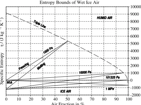
The air fraction is bound between 0 and 1 but is additionally limited by the vapour saturation condition, Fig. 5. At high total pressures, the restriction to vapour pressures below the saturation value represents a significant limitation on the upper limit of 1 – A that can be achieved in thermodynamic equilibrium. For total pressures below the vapour pressure of liquid water or the sublimation pressure of ice at the given temperature, the value of A may take any value between 0 and 1.
Fig. 4. Validity range of the Helmholtz function for humid air,
Eq. (2.7). For oceanographic and meteorological applications it is unnecessary to consider liquid or solid air. Thus, we restrict consid-eration of Eq. (4.37) as follows: (i) for temperatures above the crit-ical temperature of dry air,T >Tc=132.5306 K, all density values
occurring between the pressure bounds are permitted; and (ii) for subcritical temperaturesT <Tc, only densities below the dewpoint
curve of dry air, indicated by “Dewpoint” are permitted. The re-sulting validity boundary for dry air is shown in bold. “CP” is the critical point of dry air. To consider humid air, virial coefficients are required. The validity range in temperature of the third virial coefficients is shown by horizontal lines. Additionally, the pressure on saturated humid air is restricted to 5 MPa (Hyland and Wexler 1983), not shown.
virial coefficients are valid is from−80 to +200◦C, Fig. 4, (Hyland and Wexler, 1983). Consequently, the most limit-ing conditions for the validity of Eq. (2.7) are the tempera-ture restrictions on the viral coefficients and the requirement for validity of the truncated virial expansion, i.e. the omit-ted terms offAVproportional toA3(1−A)ρ3,A2(1−A)2ρ3 andA(1−A)3ρ3must be negligibly small in comparison to the retained terms. A rough estimate for a maximum valid density is 100 kg m−3as concluded from a comparison with experimental data for saturated air in which substantial frac-tions of both vapour and air are present (Feistel et al., 2010a; Fig. 8). When significant amounts of both air and water vapour are present, the valid temperature range is determined by the validity range for the virial coefficients. As the den-sity of either the air or vapour component is decreased, the contribution from the virial coefficients decreases and the va-lidity range in temperature extends to higher values, reaching 873 K when water vapour is eliminated and 1273 K when air is eliminated.
The air fraction is bound between 0 and 1 but is addition-ally limited by the vapour saturation condition, Fig. 5. At high total pressures, the restriction to vapour pressures below the saturation value represents a significant limitation on the upper limit of 1−Athat can be achieved in thermodynamic
0 10 20 30 40 50 60 70 80 90 1000
10 20 30 40 50 60 70 80 90 100 A ir F ra ct io n in %
Temperature t/°C
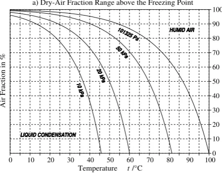
a) Dry-Air Fraction Range above the Freezing Point
LIQUID CONDENSATION LIQUID CONDENSATION LIQUID CONDENSATION LIQUID CONDENSATION HUMID AIR HUMID AIR HUMID AIR HUMID AIR 101325 Pa
101325 P a 101325 P
a 101325 Pa
50 kPa 50 kP
a 50 kP
a 50 kPa 20 kP a 20 kP a 20 kP a 20 kP a 10 k
Pa 10 k P a 10 k P a 10 k Pa
-60 -55 -50 -45 -40 -35 -30 -25 -20 -15 -10 -5 096 96.5 97 97.5 98 98.5 99 99.5 100 A ir F ra ct io n in %
Temperature t/°C
b) Dry-Air Fraction Range below the Freezing Point
ICE CONDENSATION ICE CONDENSATION ICE CONDENSATION ICE CONDENSATION
HUMID AIR HUMID AIRHUMID AIR HUMID AIR
101 101 101 101 50 kPa 50 kPa 50 kPa 50 kPa
20 kPa 20 kPa 20 kPa 20 kPa
10 k Pa 10 kP a 10 kP a 10 k
Pa
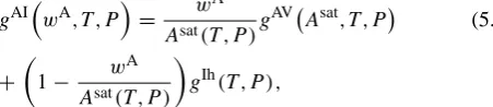
Fig. 5. Saturation curves Asat(T ,P ) of humid air at the pressures 101.325, 50, 20 and 10 kPa, as indicated. Panel (a) shows results for temperatures above the freez-ing point, computed by solvfreez-ing Eq. (5.48) usfreez-ing the library function liq air massfraction air si, Eq. (S21.9), and panel (b) shows results for temperatures below the freez-ing point, computed by solvfreez-ing Eq. (5.70) usfreez-ing the func-tion ice air massfraction air si, Eq. (S25.10). Valid air fraction values A are located above the particular satura-tion curve, A≥Asat(T ,P ), in the region indicated by “HU-MID AIR”. In the presence of ice-free seawater, the validity range forA is more restricted, A≥Acond(SA,T ,P )≥Asat(T ,P ),
by the condensation value Acond, computed from the function sea air massfraction air si, Eq. (S29.1).
equilibrium. For total pressures below the vapour pressure of liquid water or the sublimation pressure of ice at the given temperature, the value ofAmay take any value between 0 and 1.
dry f si. The Helmholtz function for air-vapour interac-tion,
fmix(A,T ,ρ)=2A(1−A)ρ RT MAMW
(2.13)
BAW(T )+
3 4ρ
A
MA
CAAW(T )+
(1−A) MW
CAWW(T )
together with its partial derivatives is implemented as the library function air f mix si. The cross-virial coef-ficients BAW, CAAW and CAWW are implemented as the
library functions air baw m3mol, air caaw m6mol2
and air caww m6mol2. The Helmholtz function of
hu-mid air, fAV(A,T ,ρ), Eq. (2.7), together with its partial derivatives is implemented as the library functionair f si. For convenience of use, some auxiliary conversion functions, Eqs. (2.9–2.12), are also implemented at level 0, Table S1. Deviating from the original formulation given by Lemmon et al. (2000), in the library the adjustable constants of dry air are specified such that the entropy and the enthalpy of dry air are zero at the standard ocean state,T=273.15 K and P=101325 Pa (Feistel et al., 2010a). This choice does not affect any measurable thermodynamic properties.
3 Level 2: Directly derived properties
From the level-one functions described in Sect. 2, various thermodynamic properties can be computed directly if the corresponding independent variables are known. If some of the input variables need to be derived first from other known ones, based on thermodynamic relations, then the function will be found at level 3 (Sect. 4) or higher.
The required input variables for level 2 functions are temperature and density of fluid pure water, either liq-uid or vapour (Sect. 3.1), temperature and pressure for ice (Sect. 3.2), and Absolute Salinity, temperature and pressure for dissolved sea salt (Sect. 3.3). For moist air, level 2 rou-tines require inputs of temperature, density and the mass fraction of (dry) air in the mixture. Specifying the air mass fraction as 1 gives the dry air limit.
The Jacobi method developed by Shaw (1935) is the math-ematically most elegant way of transforming the various partial derivatives of different potential functions into each other, exploiting the convenient formal calculus of functional determinants (Margenau and Murphy, 1943; Landau and Lif-schitz, 1964). Conversion tables (Feistel, 2008) between the potentialsf (T ,ρ),g (SA,T ,P )andh(SA,η,P )are given in
Sect. 5.
3.1 Fluid water
The total differential of the Helmholtz functionfF(T ,ρ)of fluid water has the form
dfF= −ηdT −Pdv= −ηdT + P
ρ2dρ, (3.1)
where v=1/ρ is the specific volume. Therefore, the first derivatives offFgive the specific entropy,η,
η= −
∂fF ∂T
ρ
≡ −fTF (3.2)
and the absolute pressure,P,
P = − ∂fF
∂v
T
=ρ2
∂fF
∂ρ
T
≡ ρ2fρF. (3.3)
A list of properties derived from fF(T ,ρ) by means of Eqs. (3.2) and (3.3) is given in Table S2. Partial derivatives with respect to these two independent variables are written as subscripts. Whether the property belongs to liquid water or vapour depends on the density used, i.e. on the location in the diagram in Fig. 1.
3.2 Ice
The total differential of the Gibbs functiongIh(T ,P )of ice Ih has the form
dgIh= −ηdT +vdP . (3.4)
Its first derivatives give the specific entropy,η,
η= − ∂g Ih
∂T
!
P
≡ −gTIh (3.5)
and the specific volume,v,
v= ∂g Ih
∂P
!
T
≡ gIhP. (3.6)
A list of properties derived fromgIh(T ,P )is given in Ta-ble S3. Partial derivatives with respect to the two indepen-dent variables are written as subscripts.
3.3 Dissolved sea salt
The total differential of the saline partgS(SA,T ,P )of the
Gibbs function of seawater has the form
dgS= −ηSdT +vSdP +µdSA. (3.7)
Its first derivatives give the saline part of the specific entropy, ηS,
ηS= − ∂gS
∂T
S,P
≡ −gTS, (3.8)
the saline part of the specific volume,vS,
vS=
∂gS ∂P
S,T
and the relative chemical potential, µ, µ=
∂gS ∂SA
T ,P
≡ gSS. (3.10)
The list of properties derived fromgS(SA,T ,P )is given in
Table S4. Partial derivatives with respect to the three inde-pendent variables are written as subscripts where the sub-script ofSAis omitted for simplicity.
Details on the definition of osmotic and activity coeffi-cients are given by Falkenhagen et al. (1971), Millero and Leung (1976), Ewing et al. (1994), Lehmann et al. (1996), IUPAC (1997), Feistel and Marion (2007) and Feistel (2008). The mean practical activity coefficient ln γ of sea salt (S4.1) can be computed from the activity potentialψ(S4.2) as (Feistel and Marion, 2007)
ln γ γid =
∂ (mψ )
∂m
T ,P
. (3.11)
Here, m=SA/[(1−SA)×MS] is the molality (moles of
salt per kg of water) implemented in the library as
sal molality si, andγid=1 kg mol−1is the asymptotic
value ofγ at infinite dilution. MS=31.4038218 g mol−1 is
the mean molar mass of sea salt with Reference Composi-tion (Millero et al., 2008), R=8.314 472 J mol−1K−1is the molar gas constant and (1−SA) is the mass fraction of
wa-ter in seawawa-ter. The zero-salinity limit of Eq. (3.11) is lim
SA→0
ln γ /γid=
0.
The activity potentialψ (SA,T ,P ), Eq. (S4.2), describes
the ion-ion interactions and consists of higher salinity powers O
S3A/2
of the saline part of the Gibbs function (Eq. 2.2) in the form (Feistel and Marion, 2007)
gS(SA,T ,P )=SAg2(T ,P ) (3.12)
+SARST
ln SA 1−SA
+ψ (SA,T ,P )
.
Here, RS=R/MS=264.7599 J kg−1K−1 is the specific gas
constant of sea salt. The activity potential is related to the osmotic coefficientφand the activity coefficient lnγby ψ=1−φ+ln γ
γid. (3.13)
The zero-salinity limit is lim
SA→0
ψ=0. The activity potential vanishes for ideal solutions.
The osmotic coefficientφ, Eq. (S4.11), expresses the tivity coefficient of water and can be computed from the ac-tivity potentialψ, Eq. (S4.2), as
φ=1+m
∂ψ
∂m
T ,P
. (3.14)
It is related to the chemical potential of pure water, gW (Sect. 4), and the chemical potential of water in seawater, µW, by (Feistel and Marion, 2007)
µW(SA,T ,P )=gW(T ,P )−mRT φ (SA,T ,P ). (3.15)
The zero-salinity limit is lim
SA→0
φ=1.
The saline excess chemical potential µWS, Eq. (S4.3), is the difference between the chemical potentials of water in seawater and of pure water,
µWS(SA,T ,P )=µW(SA,T ,P )−µW(0,T ,P )= −mRT φ.
(3.16) The zero-salinity limit is lim
SA→0
µWS=0.
The activity of wateraw, Eq. (S4.3), is related to the
os-motic coefficient by
aW=exp (−mMWφ)=exp (
µWS RWT
)
. (3.17)
Here, MW=18.015268 g mol−1 is the molar mass of water
(IAPWS, 2008b) andRW=R/MW=461.523 64 J kg−1K−1is
the specific gas constant of water. The zero-salinity limit is lim
SA→0
aW=1. At low vapour pressures,aWequals the relative
humidity of sea air (Feistel et al., 2010a).
The relative chemical potential µ, Eq. (S4.5), describes the change of the Gibbs energy of a seawater parcel if at constant temperature and pressure a small mass fraction of water is re-placed by salt. Its zero-salinity limit possesses a logarithmic singularity, lim
SA→0
µ=RST lnSA.
The dilution coefficient D, Eq. (S4.6), describes the change of salinity in relation to freezing or evaporation pro-cesses, (Feistel and Hagen, 1998; Feistel et al., 2010a), as e.g. in Eqs. (A28), (4.44) or (A38). The zero-salinity limit (Raoult’s law) is lim
SA→0
D=RST. The chemical coefficient
(S4.6),DS=SAD, is used for the description of sea air
(Feis-tel et al., 2010a).
The specific enthalpy, entropy and volume of sea salt, Eqs. (S4.12)–(S4.14), provide the enthalpy, entropy and vol-ume per mass of sea-salt particles dissolved in water. The zero-salinity limits are lim
SA→0
hS=g2(T ,P )−T (∂g2/∂T )P,
lim
SA→0
ηS= −RS lnSAand lim SA→0
vS=(∂g2/∂P )T. The
loga-rithmic singularity of entropy reflects the empirical fact that rigorous purification of a mixture, i.e., complete desalination, is impossible by thermodynamic processes.
Mixing enthalpy, entropy and volume, Eqs. (S4.12)– (S4.14), provide the change of enthalpy, entropy or specific volume if two seawater samples with absolute salinitiesS1,
S2and mass fractionsw1,w2are mixed at constant
tempera-ture and pressure. If the mixing occurs adiabatically at con-stant pressure, the enthalpy remains concon-stant while entropy is produced and the temperature changes. Since such effects do not occur in ideal solutions, the related quantities can be computed from the activity potentialψ (SA,T ,P )alone
3.4 Humid air
The Helmholtz function fAV(A,T ,ρ) of humid air, Eq. (2.7), permits the direct computation of all thermody-namic properties if temperatureT, densityρand air fraction Aare either given or can be obtained from similar quanti-ties such as the specific humidity,q=1−Aor the mixing ra-tior=(1−A)/A. This does not include properties at given relative humidity which requires the knowledge of vapour saturation, i.e. of the phase equilibrium between vapour and liquid water which is a composite system considered later in Sect. 5.8. A list of equations for the computation of humid-air properties from Eq. (2.7) is given in Table S5.
4 Level 3: Functions involving numerical solution of implicit equations
If quantities other than the natural independent variables of the three potential functions of Sect. 2 are given, in particular, if the pressure is known rather that the density of pure water, or the entropy rather than the temperature of seawater, the relevant thermodynamic equations must be inverted analyt-ically or numeranalyt-ically. These steps inevitably add larger nu-merical uncertainties to all properties that depend on these in-versions, and hence on the settings chosen for the associated iteration algorithms. Default values for iteration number or tolerance are specified in the SIA library routines that should be appropriate for most purposes; if necessary, they can be modified by related “set” procedures of the library (Wright et al., 2010a). Quantities that require such inversions appear in the libraries as level-3 procedures. To ensure the stability and uniqueness of the numerical solutions, initial conditions must be chosen appropriately. Various empirical functions are used to provide suitable initial values as discussed in the appendices referenced in Sect. 4.1–4.3. While the algorith-mic success and speed are sensitive to these choices, the final quantitative results are, within their numerical uncertainty, independent of the details of the initial “guess” functions. Therefore, if desired for certain applications, these auxiliary functions implemented in the library and described in this pa-per may be replaced by more suitable or effective customised ones without affecting the correctness of the final results. 4.1 Gibbs functions for liquid water and water vapour
To compute properties of fluid water at givenT andP from its Helmholtz potential, fF(T ,ρ), it is necessary to solve Eq. (S2.11),
ρ (T ,P )=g−P1, (4.1)
for the density. Except for spurious or unstable numerical so-lutions outside the validity range, Fig. 1a, there is exactly one physically meaningful solution at supercritical temperatures.
Depending on the pressure, there may be one or two stable solutions below the critical temperature, given by the inter-section points of isobars with isotherms illustrated in Fig. 1, providing the density of liquid water, ρW(T ,P ), and/or of water vapour,ρV(T ,P ).
Consequently, there cannot exist a single-valued Gibbs functiong(T,P ) that fully represents the properties of the Helmholtz functionfF(T ,ρ)of fluid water. Rather, there are two different Gibbs functions,
gW(T ,P )=fF
T ,ρW
+P /ρW (4.2)
for liquid water and
gV(T ,P )=fFT ,ρV+P /ρV (4.3)
for water vapour, which coincide under supercritical condi-tions. Interestingly, critical conditions can be encountered at hydrothermal vents in the abyssal ocean (Reed, 2006; Sun et al., 2008).
To implement the above expressions for the Gibbs func-tions we must determine the liquid and vapour densities cor-responding to the temperature and pressure inputs. This re-quires iterative solution of Eq. (4.1), with considerable care required to select the appropriate root for each case. De-tails on the iterative numerical method and the conditions used to initialize the iteration procedure are provided in Ap-pendix A1.
Once the liquid or vapour density of water is computed from the Helmholtz function fF at given temperature and pressure, the numerical values of the Gibbs function of wa-ter and its partial derivatives can be computed from the for-mulas of Table S6. The equations given there for water, gW, Eq. (4.2), apply in an analogous manner to vapour,gV, Eq. (4.3), if only the densityρof liquid water is replaced by that of vapour.
Note that the above procedure is required to ensure ar-bitrarily precise consistency between the Gibbs function of pure water and the corresponding Helmholtz function. As long as this consistency is demanded, determination of the Gibbs function and its derivatives requires an iterative nu-merical procedure to determine the density argument of the Helmholtz function, so no explicit algebraic expression is possible. Thus, the pure water component of the Gibbs func-tion must be determined at level 3 and it is only at this level that the Gibbs function for seawater can be completely de-termined. However, once the liquid pure water density is determined, the corresponding Gibbs potential is fully deter-mined and it can be used in the seawater functions described in Sect. 4.2 and 4.3.
4.2 Gibbs function of seawater
The Gibbs function of seawater, Eq. (2.1), is reproduced here as,
gSW(SA,T ,P )=gW(T ,P )+gS(SA,T ,P ), (4.4)
and is directly available from the sum of the Gibbs function of pure water computed at level 3, Table S6, and the saline part from the Primary Standard, level 1, Eq. (2.2). Properties of seawater can be computed from the partial derivatives of gSandgSWas given in Tables 4 and 7.
The Gibbs functiongSW(SA,T ,P )of seawater, Eq. (4.4),
together with its first and second partial derivatives is imple-mented as the library functionsea g si.
4.3 Enthalpy of seawater
Besides the Gibbs and the Helmholtz functions, the specific enthalpy hSW(SA,η,P ) of seawater, expressed in terms of
Absolute SalinitySA, specific entropy,η, and absolute
pres-sureP is a third important thermodynamic potential, useful in oceanography in particular for the computation of proper-ties related to adiabatic processes (Feistel and Hagen, 1995; McDougall, 2003; Feistel, 2008; IOC et al., 2010).
To compute this potential and its partial derivatives from the Gibbs functiongSW(SA,T ,P )of seawater, the
indepen-dent variableT appearing in the expression for the enthalpy,
hSW=gSW−T ∂g
SW
∂T
!
S,P
(4.5)
must be determined from knowledge of salinity, entropy and pressure. Given values ofSA, ηandP, the corresponding
value ofT is obtained by numerically solving the equation
η= − ∂g SW
∂T
!
S,P
(4.6)
to provide the implicit relationT=T (SA,η,P ). Details on
the iterative solution method used in the libraries are given in Appendix A2.
The specific enthalpy hSW(SA,η,P ) of seawater,
Eq. (4.5), as a thermodynamic potential is implemented in the library as the functionsea h si.
Once the value ofT has been determined as described in the appendix, the partial derivatives ofhSW(SA,η,P )are
ob-tained from those ofgSW(SA,T ,P )as given in Table S8.
From the enthalpy and its derivatives, all thermodynamic properties can be computed. A selection is given in Table S9 and additional quantities are given in Table S10 after so-called “potential” properties are introduced.
Many oceanic processes like pressure excursions of a sea-water parcel conserve salinity and entropy to very good ap-proximation. In particular, if a parcel is moved this way to
some reference pressureP=Pr, the thermodynamic
proper-ties given in Table S9 can be computed at that reference level from the partial derivatives ofhSW(SA,η,Pr). Such
proper-ties derived from the potential functionhSWat the reference pressure are commonly referred to as “potential” properties in meteorology and oceanography. Originally introduced by von Bezold (1888), potential temperature is defined as the temperature that a fluid parcel takes if it is moved adiabat-ically from its in situ pressure to a reference pressure level, which is often specified as the ocean surface. Analogous def-initions hold for the potential density and potential enthalpy (IOC et al., 2010).
The potential enthalpy,hθ, is obtained from Eq. (S8.2),
hθ =hSW(SA,η,Pr), (4.7)
the absolute potential temperature,θ, in K, is obtained from Eq. (S9.2),
θ= ∂h
SW(S A,η,Pr)
∂η
!
S,Pr
≡ hθη, (4.8)
and the potential density,ρθ, is obtained from Eq. (S9.1),
ρθ−1=vθ = ∂h SW(S
A,η,P )
∂P
!
S,η P
=Pr ≡ hθP. (4.9)
Evidently, for any fixed reference pressure, Pr, the values
ofhSW(SA,η,Pr)and its partial derivatives, as well as any
other arbitrary function depending on this triple of variables, remain unchanged during isentropic (η= const) and isohaline (SA= const) processes.
Derived from Eqs. (4.7) and (4.8), three kinds of thermal expansion and haline contraction coefficients are important for numerical models (IOC et al., 2010) and these are con-sidered below as the cases (i) to (vi). In these cases, we have omitted the superscripts SW on the seawater potential func-tions for simplicity of the expressions. As well, we have al-ways regarded the reference pressurePras a constant value
in each derivative considered here, without explicitly indicat-ing this in the formulas. This implies that potential enthalpy, Eq. (4.7), and potential temperature, Eq. (4.8), are pressure-independent functions of salinity and entropy, and in partic-ular, that any derivatives taken at constant (SA,η) can
equiv-alently be taken at constant (SA,θ) or constant (SA,hθ). An
example is the isentropic compressibility,
κs=−
1 v
∂v
∂P
S,η
=−1
v
∂v
∂P
S,θ
=−1
v
∂v
∂P
θ S,h
. (4.10)
(i) The thermal expansion coefficient,αT, is defined as:
αT= 1
v
∂v ∂T
S,P
It is expressed in terms of derivatives of enthalpy by means of the Jacobi method and Eqs. (S9.1), (S9.2), as
αT =1
v
∂ (v,SA,P )
∂ (T ,SA,P )
=1
v
∂ (v,SA,P )
∂ (η,SA,P )
∂ (T ,SA,P )
∂ (η,SA,P )
(4.12)
=1
v
(∂v/∂η)S,P (∂T /∂η)S,P =
hηP hPhηη
.
Using Table S8, the partial derivatives ofhcan be substituted by those ofg, with the result
αT = hηP
hPhηη
=gT P
gP
. (4.13)
(ii) The thermal expansion coefficient with respect to poten-tial temperature,αθ, is defined as:
αθ= 1
v
∂v
∂θ
S,P
(4.14)
Similar to Eq. (4.12), with the help of Eq. (4.8) we compute αθ= 1
v
∂ (v,SA,P )
∂ (θ,SA,P )
=1
v
∂ (v,SA,P )
∂ (η,SA,P )
∂ (θ,S A,P )
∂ (η,SA,P )
(4.15)
=1
v
(∂v/∂η)S,P (∂θ/∂η)S,P =
hηP hPhθηη
.
Using Table S8, the partial derivatives ofhcan be substituted by those ofg, with the result
αθ= hηP
hPhθηη
= gT Pg
θ θ θ gPgT T
. (4.16)
Here, gθ is the potential Gibbs energy defined as gθ≡
g (SA,θ,Pr).
(iii) The thermal expansion coefficient with respect to po-tential enthalpy,αh, is defined as:
αh=1
v
∂v
∂hθ
S,P
(4.17)
Similar to Eq. (4.12), with the help of Eq. (4.7) we compute αh=1
v
∂ (v,SA,P )
∂ hθ,S A,P
=1
v
∂ (v,SA,P )
∂ (η,SA,P )
∂ hθ,S A,P
∂ (η,SA,P )
(4.18)
=1
v
(∂v/∂η)S,P ∂hθ/∂η
S,P
= hηP
hPhθη .
Using Table S8, the partial derivatives ofhcan be substituted by those ofg, with the result
αh= hηP
hPhθη
= − gT P
gPgT T θ
. (4.19)
The thermal expansion coefficient with respect to conser-vative temperature, α2, is related to Eq. (4.19) by a con-stant conversion factor,c0P=3991.86795711963 J kg−1K−1,
asα2=c0Pαh (IOC et al., 2010). Conservative temperature, 2, is potential specific enthalpy,hθ, Eq. (4.7), expressed in terms of an arbitrarily defined temperature unit,2=hθ/c0P (McDougall, 2003; IOC et al., 2010); as such, it belongs to level 5 of the library where non-basic-SI units and user-defined functions are implemented. In contrast, potential en-thalpy itself is defined at the core level 3 of the SIA library.
(iv) The isothermal haline contraction coefficient,β, is de-fined as:
β= − 1
v
∂v
∂SA
T ,P
. (4.20)
Similar to Eq. (4.12) we write Eq. (4.20) in terms of Jaco-bians
β=−1
v
∂ (v,T ,P ) ∂ (SA,T ,P )
=−1
v
∂ (v,T ,P ) ∂ (SA,η,P )
∂ (S
A,T ,P )
∂ (SA,η,P )
.
(4.21) Expanding the functional determinant in the numerator yields, with the help of Eqs. (S9.1) and (S9.2)
β= −1
v
∂v ∂SA
η,P
∂T ∂η
S,P
−∂v
∂η
S,P
∂T ∂SA
η,P
∂T ∂η
S,P
(4.22)
= − 1
hP
hSPhηη−hηPhSη hηη
.
Using Table S8, the partial derivatives ofhcan be substituted by those ofg, with the result
β=hSηhηP −hSPhηη
hPhηη
= −gSP
gP
. (4.23)
(v) The haline contraction coefficient with respect to poten-tial temperature,βθ, is defined as:
βθ = − 1
v
∂v
∂SA
θ,P
(4.24)
Similar to Eq. (4.12) we write Eq. (4.24) in terms of Jaco-bians
βθ=−1
v
∂ (v,θ,P ) ∂ (SA,θ,P )
=− 1
v
∂ (v,θ,P ) ∂ (SA,η,P )
∂ (SA,θ,P )
∂ (SA,η,P )
. (4.25) Expanding the functional determinant in the numerator yields, with the help of Eqs. (S9.1) and (S9.2)
βθ = − 1
v
∂v ∂SA
η,P
∂θ ∂η
S,P
−∂v
∂η
S,P
∂θ ∂SA
η,P
∂θ ∂η
S,P
(4.26)
= − 1
hP
hSPhθηη−hηPhθSη hθ
ηη
Using Table S8, the partial derivatives ofhcan be substituted by those ofg, with the result
βθ=h
θ
SηhηP−hSPhθηη hPhθηη
=gT P gST
−gSθθ −
gSPgT T gPgT T
. (4.27)
(vi) The haline contraction coefficient with respect to poten-tial enthalpy,β2, is defined as:
β2= − 1
v
∂v
∂SA
hθ,P
(4.28)
Similar to Eq. (4.12) we write Eq. (4.28) in terms of Jaco-bians
β2= − 1
v
∂ v,hθ,P ∂ SA,hθ,P
(4.29)
= − 1
v
∂ v,hθ,P ∂ (SA,η,P )
/∂ SA,h θ,P
∂ (SA,η,P )
.
Expanding the functional determinant in the numerator yields, with the help of Eq. (4.7)
β2= − 1
v
∂v ∂SA
η,P
∂hθ ∂η
S,P
−
∂v ∂η
S,P
∂hθ ∂SA
η,P
∂hθ ∂η
S,P
(4.30)
= − 1
hP
hSPhθη−hηPhθS hθ
η .
Using Table S8, the partial derivatives ofhcan be substituted by those ofg, with the result
β2=h
θ
ShηP−hSPhθη hPhθη
=gSTgT P−gSPgT T−g
θ SgT P/θ gPgT T
.
(4.31) The latter equalities in Eqs. (4.13), (4.16), (4.19), (4.23), (4.27) and (4.31) are the results given earlier in Table S7. The potential quantities written in terms of the enthalpy of seawater are listed in Table S10.
Entropy as a function of salinity, temperature and pressure is available from Eq. (S7.2). Potential temperature is defined by the relationη(SA,T ,P )=η(SA,θ,Pr), therefore the same
function (Eq. S7.2) can be used to compute entropy as a func-tion of salinity, potential temperature and reference pressure. Since the cases (i) to (vi) above, Eqs. (4.13), (4.16), (4.19), (4.23), (4.27) and (4.31), specify the different expansion and contraction coefficients as functions of entropy, these coeffi-cients are available as functions of potential temperature, too, by means of Eq. (S7.2).
From the enthalpy definition Eq. (4.5) and the differential Eq. (3.7) of the Gibbs function, the relation
dηSW= 1
Tdh− v
TdP − µ
TdSA (4.32)
can be inferred. Hence, when enthalpy is used as an inde-pendent thermal variable in combination with salinity and pressure, the responsible thermodynamic potential function is entropy,ηSW(SA,h,P ). Note that the superscript “SW”
onηis included here to indicate its use as a thermodynamic potential function for seawater, consistent with the inclusion of “SW” on both the Gibbs functiongSW and the enthalpy hSWwhen used as a potential function for seawater. To ob-tain this function value numerically from its arguments, the Eq. (S8.2)
h=hSW(SA,η,P ) (4.33)
must be solved forη. Because of Eq. (4.7), if the potential enthalpy valuehθ is given, the same algorithm can be used to get the related entropy from
hθ =hSW(SA,η,Pr). (4.34)
The inversions of Eqs. (4.33) and (4.34) give respectively
η=ηSW(SA,h,P ) (4.35)
and
η=ηSW SA,hθ,Pr, (4.36)
which are really the same functions with different ar-guments. The iterative inversion algorithm is straight forward and is implemented as the library function
sea eta entropy si. It provides entropyηin the form of eitherηSW(SA,h,P )or ηSW SA,hθ,Pr, from which in
turn all properties listed in Tables S9, S10 can be determined. Note, however, that we have not implemented an explicit routine for entropy, Eq. (4.35), as a potential function in the library. That is, the functionsea eta entropy si pro-vides entropy as a function of salinity, enthalpy and pres-sure, but it does not provide the partial derivatives of entropy with respect to those variables, nor does it take any orders of derivatives as input parameters. As such, the thermodynamic potential “entropy” is not available in the present SIA library version in the same form as the other potential functions that are summarised in Table 1. Nevertheless, various properties (Tables S9, S10) derived from it are implemented at level 3 and evaluated from indirect algorithms, just as if the potential “entropy” were available. The corresponding routines can be identified in the implementation of the library discussed in Part 2 (Wright et al., 2010a) by an eta instead of an h
in the function names given in Table S10, which indicates the implicit use of entropy as the potential function. Conse-quently, these routines take enthalpy or potential enthalpy as the thermal input parameter rather than entropy.
4.4 Gibbs function of humid air