27
International Journal of Integrated Engineering (Issue on Civil and Environmental Engineering)
Modelling Thermal Environmental
Performance In Top-lit Malaysian
Atrium Using Computational Fluid
Dynamics (CFD)
A.H. Abdullah1,* and F. Wang2
1Faculty of Civil and Environmental Engineering, Universiti Tun Hussein Onn Malaysia, Malaysia
2School of the Built Environment, Heriot-Watt University, Scotland, United Kingdom *Corresponding email: [email protected]
Abstract
Computational Fluid Dynamics (CFD) programs are powerful design tools that can predict
detailed flow movement, temperature distribution, and contaminant dispersion. This paper
reports the steady-state 3-D CFD modelling of air movement and temperature distribution due to thermal buoyancy within top-lit three-storey representative Malaysian atrium
forms using the computer code PHOENICS. Details of temperature distribution, airflow
patterns and other comfort parameters would provide a better picture of the resultant thermal performance within the atrium in response to the changes of design variables. The CFD modelling studies were to investigate quantitatively the effects of varying inlet to outlet opening area ratios and also the outlet’s arrangement on the atrium’s thermal environmental performance in relation to occupants’ thermal comfort. The simulation
results have revealed that sufficiently higher inlet to outlet opening area ratio (i.e. n>1)
can improve the thermal performance on the occupied levels; while with an equal inlet to outlet opening area ratio (i.e. n=1), changing the outlet’s arrangement (i.e. location and
configuration) has not significantly affected the atrium’s thermal performance.
1. INTRODUCTION
Application of Computational Fluid Dynamics (CFD) in the built environment
particularly modelling room air flow for
the design of indoor climate control has matured greatly in the last few years. Such CFD programs are proven useful at all stages of the design, offering increased accuracy and cost effectiveness over empirical and scale modelling techniques [1]. In the
field of building services engineering the
techniques are used increasingly to conduct studies in performance assessment of building ventilation, air quality, occupant comfort etc.
Indoor air flow is characterized by
low velocity and high turbulence intensity. When applying CFD to the study of indoor
airflow and thermal environmental quality,
it is to numerically model physical processes
occurring within a fluid by the solution
of a set of non-linear partial differential equations (i.e. Navier-Stokes equations). These partial differential equations express the fundamental physical laws that govern the conservation of mass, momentum and
thermal energy to a control volume of fluid
[2].
Simulating the flow field in large
enclosure such as atria with CFD is
generally more difficult to model than conventionally-sized enclosures. As the
space is large, one is forced to carry out a simulation with larger computational cells due to limited computing capacity. A coarser grid will not only result in various types of numerical errors but also produce an inaccurate modelling of the turbulent
flow field.
Using the computer code PHOENICS (version 3.6.1), the parametrical studies were carried out to investigate quantitatively
the effects of some critical aspects of
ventilation openings (i.e. size, location and configuration) on the thermal environmental
performance within the top-lit three-storey representative Malaysian atrium form. Some of the computed indoor thermal environmental variables such as air and resultant temperatures, and air movement were used to evaluate and compare the resulting thermal environmental performance within the central atrium with regard to the users’ thermal comfort.
As reported by Sabarinah [3], Ismail and Barber (2001) suggested that Malaysian atria can be habitable or thermally comfortable when the indoor resultant temperature and relative humidity within the occupied levels range between 20.8-28.6ºC and 40-80%, respectively, in air-conditioned space. As for the naturally ventilated indoor space, however, the maximum range can be increased slightly depending on the air movement (i.e. generally between 0.5-1.0 m/s) and activity level.
29
International Journal of Integrated Engineering (Issue on Civil and Environmental Engineering)
conditions which are near thermal neutrality (slight discomfort). A space is therefore considered to be thermally comfortable when the PMV values are between –2 and +2, as recommended by Fanger [4] and ISO 7730 [5].
2. GENERAL DEVELOPMENT
AND SPECIFICATIONS
OF CFD ATRIUM MODEL
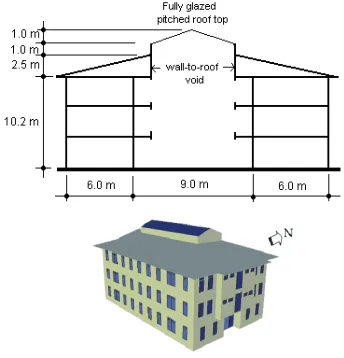
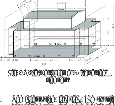
The general design characteristics of the 3-D CFD model and thermo physical characteristics of air and boundary conditions were kept identical to those simulated earlier with dynamic thermal modelling software TAS. Fig. 1 shows the simulated 3-D TAS top-lit Malaysian atrium model and its cross-section.
Fig. 1 The simulated 3-D TAS atrium model
2.1 Domain
Basically, the interest of this study was to examine the air distribution and vertical temperature gradients within the atrium
well. Therefore, the numerical domain was
only confined to the central linear atrium which includes ground floor level, first and second floor balcony and corridor areas, as
well as wall-to-roof void and below roof
areas. As such the adjacent floors were not included in the numerical domain. The size
of the numerical domain in terms of length, width and height was 30 m × 9 m × 14.7 m. In order to consider only the void areas
within the central atrium, the flow domain was further defined by creating blockage
objects at the four corners of the three occupied levels and also the areas above the occupied levels surrounding the wall-to-roof void and below roof areas as shown
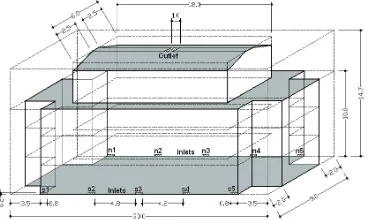
in both Figures 2 and 3. The fully glazed
pitched roof top for the top-lit model was created using two wedge-shaped objects
and slightly modified with a flat plate object sized 1.0 m wide and 18 m long at its
pitch. This was purposely done in order to accommodate for the central rooftop vent (outlet), which was otherwise impossible to be located with fully pitched rooftop due to the wedge-shaped objects.
2.2 Boundary Conditions
The solution domain was bounded by
solid surfaces (including walls, floor, ceiling and/or roof and glazing) and fluid
surfaces (such as air supply and exhaust openings). Correct information on the effect of solar absorptions at the internal surrounding surfaces, which directly affect the indoor air temperature due to the high heat energy, is essential when simulating thermal environment in highly
glazed enclosures. The data predicted by
dynamic thermal simulation, TAS model,
hourly climatic effects (i.e. solar radiation, wind speed and direction, temperature and humidity), operational effects (i.e. heat gains from people, light, and equipment; and HVAC system performance), and building elemental conditions were taken into account.
The dynamic thermal simulations
were carried out using 1978-weather file
for Subang, Kuala Lumpur for day 80 (21st March), representing the hottest design day of the year for Malaysia as suggested by many authorities [6, 7, 8]. As such, based on the conditions and results from the dynamic
thermal modelling (TAS) of ground floor
only pressurised simulations, the boundary conditions applied to the top-lit CFD atrium model can be outlined as follows:
• The internal temperatures of the
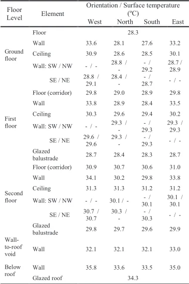
boundary surfaces were taken from the dynamic thermal simulation results of elemental surface temperatures at 1400 hr (i.e. the hottest hour of the day) as detailed in Table 1. Indoor thermal conditions at 1400 hr are to represent the atrium’s worst-case scenario.
• The net heat input, Qs, (or surplus heat)
inside the atrium, which is the net heat gain (i.e. from occupants, lighting, solar, etc.) minus the heat losses (due to heat transmission through surfaces
and infiltration), were estimated using
Equation (1) [9, 10]: V1 = 0.037(QsH1)1/3 (C
d1A1)1/2 (1) where;
V1 : the total supply air flow (i.e. 3.36
m3/s),
Qs : the net heat input, H
H1 = ––––– : where H1 is the vertical 1 + n2
distance from the centre of inlet opening to the neutral pressure plane level, and H is the vertical distance from the centre of inlet opening to the centre of outlet opening (i.e. 14.6 m); and n2 = (T
ai/Tao)(A1/A2)2 where Tai is the
average atrium indoor air temperature at 1400 hr (i.e. 26.89 ºC)and Tao is the supply air temperature at inlets (which was 23ºC), and the total inlet (A1) and outlet (A2) opening areas were similar to those of TAS modelling (i.e. A1 = 4 m2 and A
2 = 10 m).
Cd1 : discharge coefficient for inlet
(= 0.57).
Table 1: Elemental surface temperatures for CFD model
Floor
Level Element
Orientation / Surface temperature (ºC)
West North South East
Ground floor
Floor 28.3
Wall 33.6 28.1 27.6 33.2
Ceiling 30.9 28.6 28.5 30.1
Wall: SW / NW - / - 28.8 / - 29.2 - / 28.7 / 28.9
SE / NE 28.8 / 29.1 28.4 / - 28.7 - / - / -
First floor
Floor (corridor) 29.8 29.0 28.9 29.8
Wall 33.8 28.9 28.4 33.5
Ceiling 30.3 29.6 29.4 30.2
Wall: SW / NW - / - 29.3 / - 29.3 - / 29.3 / 29.3
SE / NE 29.6 / 29.6 29.3 / - 29.3 - / - / -
Glazed
balustrade 28.7 28.4 28.3 28.7
Second floor
Floor (corridor) 30.9 30.7 30.6 31.0
Wall 34.1 30.2 29.8 33.8
Ceiling 31.3 31.3 31.2 31.2
Wall: SW / NW - / - 30.1 / - 30.1 - / 30.1 / 30.1
SE / NE 30.7 / 30.7 30.3 / - 30.3 - / - / -
Glazed
balustrade 29.8 29.7 29.6 29.9
Wall-to-roof
void Wall 32.1 32.1 32.1 33.0
Below
roof Wall Glazed roof 35.8 33.6 34.3 33.5 35.0
31
International Journal of Integrated Engineering (Issue on Civil and Environmental Engineering)
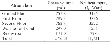
• It was also assumed that the net heat
input, Qs, was uniformly distributed within the atrium well and the estimated net heat input at 1400 hr for
each atrium level (which was specified
according to its volume) is summarised in Table 2.
Table 2 : Estimated net heat input, Qs, (in Watt) within the atrium at 1400 hr
In atria, the airflow is typically
predominantly thermally driven since the momentum of supply jets diminishes with throw distances and the momentum of buoyant plumes increases with height [11].
The atrium fills with warm air due to the
net heat input, Qs, and the deep warm layer between ventilation openings (i.e. inlet and outlet openings) located at different levels
enhances the flow [12]. In this modelling,
the atrium ventilation by thermal buoyancy was obtained by providing low-level inlet
openings supplying cooler 23˚C air into the ground floor atrium and high-level outlet
opening to exhaust the hot air out of the atrium.
2.3 Turbulence Model
The indoor airflow is usually a turbulent flow. The Reynolds numbers (the ratio of inertia to viscous forces) for most flows
within the built environment are in the transition range. Even in the turbulent regime, there is currently no universal
turbulent model available that can reflect
the behaviour of full range of complex
turbulent flows observed in buildings.
From the viewpoint of engineering use,
simulation based on the Reynolds averaged equation is the most efficient and commonly
used. The k-ε two-equation model is used to incorporate the effect of turbulence on
the flow. The model was first developed
by Harlow and Nakayama [13] and further
refined by Launder and Spalding [14].
The standard k-ε turbulence model has been widely applied in predicting
many types of turbulent flow phenomena
including ventilation design applications, yielding many satisfactory results [15, 16, 17]. For these CFD simulations, therefore,
the standard k-ε turbulence was applied with the HYBRID differencing scheme
in combination with the standard
wall-function. The log-law velocity profile was
imposed at the inlet boundary, no-slip rough wall surface on the ground of the domain
whereby no flow through this surface and shear velocity on it remains zero, and zero
static pressure at the outlet.
2.4 Radiation Model
In the study of airflow and heat transfer in
a large enclosure, it is essential to consider surface heat exchange not only by natural convection but also by long-wave thermal radiation (infrared radiation) [11]. Both these phenomena are governed by surface temperature. In a large indoor space such as an atrium, the ceiling’s surface temperature may be affected by pronounced thermal
stratification, such that the radiative heat flux from the areas below the roof to
other surfaces is very large. Similarly, as
the floors and walls are heated by solar
Atrium level Space volume (m3) Net heat input, Q
s (Watt)
Ground Floor 755.8 3195
First Floor 789.3 3336
Second Floor 762.3 3222
Wall-to-roof void 297.0 1255
Below roof 171.0 723
radiation, the absorbed heat is redistributed to other surfaces by long-wave radiation. Therefore, the long-wave redistribution of solar radiation in this way is vital to be considered in this CFD atrium modelling studies.
The radiative heat transfer within the representative atrium models was solved
by radiation model called IMMERSOL. The IMMERSOL method involves
three main elements as follows [POLIS: the PHOENICS On-Line Information System]:
• Solution for the variable T3 , from
a heat-conduction-type equation with a local conductivity dependent on the nature of the medium, on its temperature, and on the distance between nearby solid walls.
• Solution for the temperature of the fluid phase(s) by means of the
conventional energy equation(s), having either temperature or enthalpy as the dependent variable(s).
• Modifications of the source terms, in
cells adjacent to solids, which account for the departures of the surface emissivity from unity.
Settings for IMMERSOL radiation
model should be made in order to activate solution for the required variables. For these CFD simulations, the absorption
coefficient was set to be 1.0 and the ‘Store Radiative energy fluxes’ was switched ON.
The emissivity of all the boundary surfaces was also set in addition to their surface temperatures. The internal walls which were
of plastered bricks and the concrete floor
elements were set to have emissivity of 0.9,
whereas the emissivity of glazed walls and
roof elements were set to be 0.845.
2.5 Grid Density
An orthogonal grid based on the Cartesian
coordinate system (x,y,z coordinate axes)
was employed in these simulations. As the atrium enclosures were large, it is essential
to use finer grid near boundary surfaces in order to more accurately bridge the flow field with the boundary conditions for flow
and heat transfer.
The airflow in the atrium space
was driven by forced convection due to pressurised ventilation air from the
surrounding offices, and by natural
convection due to differing wall surface temperatures. In order to accurately predict
the flow field inside the atrium dominated
by forced convection, it was important to reproduce precisely the jet stream from each inlet [11]. The jet goes through a mixing process, entraining the surrounding air and mixing with it. The large velocity gradient which was formed in this mixing region produced much turbulence. The jet’s diffusion pattern therefore greatly depends on the velocity gradient and the accompanied turbulence. The accuracy of predicting this pattern nearly entirely depends on the accuracy of reproducing the velocity gradient within the boundary layer, which is subjected to the local grid
size. Thus, the grid size in the jet region must be very fine.
The airflow through outlet opening has practically no effect on the air flow pattern within the atrium. It can be assumed a zero
gradient normal to the outlet opening for all
the flow variables. Consequently, the local grid size has little effect on the accuracy of enclosure’s airflow distribution.
In addition, accurate treatment of
near-wall flow (boundary layer flow) is
33
International Journal of Integrated Engineering (Issue on Civil and Environmental Engineering)
accurate solution of the airflow in the core of the atrium. On the ground floor where
pressurised air was introduced through the inlets, a steep velocity gradient is form next to each wall, due to friction, with
zero velocity at the wall surface. These are
described as forced-convection boundary layers. Furthermore, within the atrium where the wall surface temperature is
generally high, the influence of temperature
becomes predominant, and a thin layer of rising and falling buoyant air develops along walls (surfaces facing the enclosure,
including the floor and ceiling). These are
described as natural-convection boundary layers. As the boundary layer is typically only several millimetres thick, it is very important that the loss of velocity and heat transfer mechanism in this thin layer be
accurately dealt with by using very fine
grid near the wall.
As the discretized domain was large
and bearing in mind the computing cost of very dense grid, it is very important to have the right or necessary amount of grid points (cells) to optimise the simulation. The numerical tests on grid-independence had been carried out, and it was decided that the mesh of 180×64×90 (i.e. 1,036,800 cells) is fairly reasonable to capture the heat and air exchanges within the enclosure.
2.6 Iteration Number
Apart from having sufficient numerical grid
points and resolution, the accuracy of the solution obtained by CFD simulation also usually depends on the degree to which the
solution satisfies the discretised equations.
This can normally be assessed by the level of imbalanced error-sources within discretised equations. Most commercial
CFD software packages incorporate a graphical representation of these sources, which gives a useful indication on convergence.
A point in a flow domain at which the flow variables can be probed or monitored
as the solution runs should be carefully set. In general, the probe is positioned at a
location where flow is expected to have a
high value of velocity gradient. Particularly
in a large flow domain, a few trial runs
should be carried out to identify the most critical location that affect the overall
solution of the flow field parameters in
the domain. At this critical monitoring
point it is normally rather difficult to get
converging solution and usually requires longer running time (or higher iteration number) for the values of the variables to become stable or constant. From the trial runs, it was decided that the probe position should be located at IXMON=131 (location of cell along x-axis), IYMON=48 (location of cell along y-axis), and IZMON=68
(location of cell along z-axis).
As the right amount of computational grid cells and probing position have been determined, the convergence tests was then carried out. Using Intel Pentium 4 CPU
(2.00 GHz) with 1,039,896 KB RAM, it
was observed from the ‘Solver’ run screen that the values of all the solved variables converged to stable levels with their residual errors dropped to minimum as the iterations approached 1500.
3. PARAMETRICAL STUDIES
This modelling study investigated quantitatively the effects of varying both the inlet to outlet area ratios and outlet’s
of outlet section) on the atrium’s thermal environmental performance. Additional CFD model descriptions for each of the parametrical studies are described in the following sub-sections. The resulting atrium’s thermal environmental performance in relation to users’ thermal comfort for each design variable investigated was basically assessed based on the predicted air and resultant temperatures, air movement, and ‘Predicted Mean Vote’ (PMV) index.
3.1 Varying Opening Area Ratio
For a higher indoor space, the neutral pressure plane is a certain level between inlet and outlet openings where the inside and outside pressures are equal. Below the neutral pressure plane there will be an indoor negative pressure allowing an inward
airflow through the inlet, whilst above the
neutral pressure plane there will be positive
pressure forcing the room air to flow out
through the outlet. The development of CFD atrium model to investigate quantitatively the effects of varying the inlet to outlet opening area ratios on the atrium’s thermal environmental performance are outlined as follows:
• Based on the equation, n2 = (T
ai/Tao)(A1/ A2)2, the changes of the neutral pressure plane are essentially dependent on changes of the ratio of total inlet area to total outlet area (A1/A2) as is almost constant. Thus, n ≈ A1/A2. This study examined three different inlet to outlet area ratios such as n = 0.5, n = 1, and n = 1.6. Smaller inlet to outlet area ratio (i.e. A1≤A2) implies higher neutral pressure plane level causing higher inlet velocity. On the contrary, greater inlet to outlet ratio (i.e. A1>A2) would
bring down the neutral pressure plane level resulting in smaller inlet velocity associating with smaller ‘driving force’ through the inlets.
• The total inlet opening area was fixed
to be 1.6 m2. It was assumed that the
23˚C air was supplied through ten low-level inlet openings sized 0.8 m long
by 0.2 m high located on both north
and south walls of the ground floor
atrium (see Fig. 2).
The 3.36 m3/s total air volume
flow were supplied through the ten
inlets with each inlet equally supplying 0.336 m3/s.
• As the total inlet area was fixed at
1.6 m2, the total outlet opening area was calculated based on the inlet to outlet area ratio, n. The outlet opening area for each value of n and its associated
size and location are summarised in
Table 3 and illustrated in Fig. 2.
• The comfort index calculation,
particularly for dry resultant temperature and ‘Predicted Mean Vote’ (PMV), was also activated. The software computed dry resultant temperatures by solving air temperature, radiant temperature
and the velocity of airflow at any
location within the enclosure based on the given physical boundary conditions of surface temperatures, net heat input
and the supply air flow rate.
• In addition to the solved air
35
International Journal of Integrated Engineering (Issue on Civil and Environmental Engineering)
Clo-value and metabolic rate were set to be 1.0 (typical business suit) and 2.0 (2 km/hr walking on level), respectively, representing the typical clothing worn
by people in an office building and
also their common activity (in addition to seated quietly and standing at ease) within the atrium.
The relative humidity was set to be 80%. The higher relative humidity setting compared to the value
recommended by ASHRAE and other organisations was to reflect the fact that
Malaysians are acclimatised to much higher environmental temperature and humidity level [3]. Furthermore, the atrium is generally used as a relaxing, transitional space, which requires less stringent indoor comfort conditions.
Fig. 2 CFD atrium models showing low-level inlet and high-level outlet sizes due to different
opening area ratios
Table 3 : The size and location of high-level outlet opening due to different opening area
ratios
(a) n = 0.5
(b) n = 1.0
(a) n = 0.5
(b) n = 1.0
Area
ratios (n) Outlet opening area (m2) Outlet opening size location
0.5 3.2 3.2 x 1.0 m Central
glazed rooftop
1.0 1.6 1.6 x 1.0 m
1.6 1.0 1.0 x 1.0 m
3.2 Varying Outlet’s Arrangement
This parametrical study was to examine quantitatively the effect of outlet’s
arrangement (i.e. location and configuration)
on atrium’s thermal environmental performance. The resulting performance of
existing horizontal central rooftop vent for
the top-lit model was compared with that of vertical side vent. Additional descriptions of CFD atrium model for this study are outlined as follows:
• The inlet to outlet area ratio of 1.0
(i.e. n=A1/A2=1.0) was used for these simulations. Hence, the total outlet opening area was 1.6 m2 as the
total inlet opening area was fixed at
for central rooftop vent was similar to that shown in Fig. 2b. Fig. 3 shows
the size, location, and configuration
of the outlet opening for top-lit model with side vent. The 3.2 m long by 0.5 m high vertical outlet opening section was located at the central top of the north clerestory walls.
Fig. 3 Outlet’s arrangement with vertical side vent
• The inlets’ size, location, and supply air volume flow rate were exactly the
same as that of the study on the effect of varying the ratios of inlet to outlet opening area described in section 3.1.
• Comfort indices activation and
settings for this simulation were also maintained to be similar to those of section 3.1.
4. RESULTS AND DISCUSSION
Apart from data on average indoor air temperature within each particular atrium level, the average air velocity, resultant temperature, and pressure gradient will also be used in analysing and discussing the thermal environmental performance within the atrium. In addition, the sectional
plots of the computed variables including PMV index will be included for better visualisation of the overall atrium’s thermal performance. When the plot of the variables is used, the probe position is generally located at the centre of the atrium on the top occupied level at the
height of 1.7 m from its floor level. This
middle level is purposely chosen because it represents the average height of a person or slightly above the body level of a tall person. Hence, this level is assumed to be most sensitive to the users’ sensation of thermal comfort.
4.1 Effects of Opening Area Ratio on Thermal Performance
Varying the inlet to outlet area ratios would result in the changes of the neutral pressure plane level. Consequently this would affect the thermal environmental performance within the enclosure. Fig. 4b shows the vertical pressure gradient and the resulting neutral pressure plane levels associated with the inlet to outlet area ratios.
Fig. 4 Average air temperatures and pressure gradient due to different opening
area ratios
0 2 4 6 8 10 12 14 16
24 25 26 27 28 29 30
Temperatures (C)
Height (m)
n=0.5 (A1=1.6; A2=3.2) n=1 (A1=1.6; A2=1.6) n=1.6 (A1=1.6; A2=1.0)
-16 -12 -8 -4 0 4 8 12 16
Pressure (Pa)
n=0.5 (A1=1.6; A2=3.2) n=1 (A1=1.6; A2=1.6) n=1.6 (A1=1.6; A2=1.0)
37
International Journal of Integrated Engineering (Issue on Civil and Environmental Engineering)
Fig. 4a shows the average air temperatures within the central atrium due to the total inlet to outlet opening area
ratios of 0.5, 1.0, and 1.6 (with the fixed
total inlet opening area of 1.6 m2). It can be seen from the graph that the differences in the average air temperature between each of the area ratios were very small. The main reason for these slight differences was probably due to the relatively small differences between the total inlet area and the outlet area for the large atrium volume.
Furthermore, Fig. 4a also exhibits that the resultant thermal performance within the representative atrium models for both opening area ratios, n=0.5 and n=1.0, were very much similar to each other. Their higher neutral pressure plane level, which can be clearly seen from Fig. 4b, led to the increase in the pressure difference across the inlets. Therefore, as a result of slightly higher inlets’ velocity due to greater ‘driving force’ through the inlets, the indoor air particularly within the occupied levels was well-mixed. In general, the simulation results showed that the average air velocity on occupied levels for both area ratios of n=0.5 and n=1.0 were slightly higher than that of the area ratio n=1.6. On the other hand, the higher neutral pressure plane level lead to the decrease in the ‘driving force’ through the outlet; thereby, slightly lowering the average air velocity within the wall-to-roof void and below roof areas, which further reduced the ventilation capacity at the outlet (refer to Fig. 5b). The well-mixed hot indoor
air coupling with lower outward flow rate of the stratified hot air in the below
roof areas due to higher neutral pressure plane level were the main reasons for
0 2 4 6 8 10 12 14
0.02 0.04 0.06 0.08 0.10 0.12 0.14 0.16 Air Velocity (m/s)
He
ig
ht
(m
)
n=0.5 (A 1=1.6; A 2=3.2) n=1 (A 1=1.6; A 2=1.6) n=1.6 (A 1=1.6; A 2=1.0)
1 ––2
causing such similar thermal conditions for both opening area ratios, n=0.5 and n=1.0.
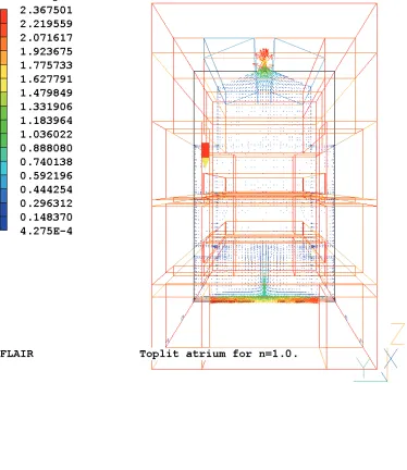
Fig. 5 Vector plot of air velocity for area ratio, n=1.0 and average air velocity due to different
opening area ratios
However, it also can be seen from Fig. 4a that the thermal performance within the atrium model was slightly better for opening area ratio, n=1.6. These results very well satisfy Equation (2), the expression for supply ventilation rate as formulated by Andersen [9, 10].
2gH1∆T
V1 = Cd1A1 –––––––––– (2)
As the supply ventilation rate, V1, and
the net heat input, Qs, were kept constant,
thus, lowering H1 (i.e. shorter vertical distance from the centre of inlet opening to the neutral pressure plane level) would reduce the indoor air temperature, Tai.
Similarly, temperature difference, ΔT,
would also be lower and this would further decrease the pressure difference across the inlet. Smaller ‘driving forces’ through the inlets led to slightly lower inlets’ velocity. Higher ‘driving force’ through the outlet also helped to increase the ventilation capacity at the outlet which further
enhanced the outward flow of the stratified
hot air, particularly in the below roof areas (Fig. 5b).
In general, the average air velocity in the below roof area was higher when the opening area ratios was greater than 1.0 due to the higher ventilation capacity through the outlet. However, it can be clearly seen from Fig. 5 that the average air velocity at upper levels particularly
from first floor level to wall-to-roof void
level was very low, which was generally less than 0.045 m/s. As the cooled air was discharged at low level, the
temperature stratification at upper levels
was highly stable. Consequently, the vertical air movement was greatly
suppressed causing the airflow to become stagnant particularly on the first floor level, second floor level and wall-to-roof
void area. This is undesirable, as it would
drive the stratified hot air to flow in to top
occupied level making the surrounding area hot and uncomfortable.
It should be noted that Equation (2) is valid only if the position of the neutral pressure plane level is not below the upper edge of the inlet or above the lower edge
of the outlet. The vertical distance from the centre of inlet to the neutral pressure plane level, H1, influences the ventilation capacity
through the inlet and also inlet’s velocity. Likewise, the vertical distance from the neutral pressure plane level, H2, to the
centre of outlet influences the ventilation
capacity through the outlet and also outlet’s velocity. Therefore, low neutral pressure plane level can be achieved
by sufficiently high inlet to outlet area
ratio.
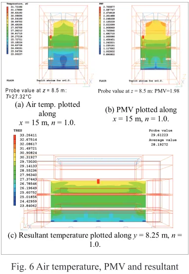
The resulting thermal environmental performance within the top-lit atrium model can be seen in Fig. 6. The thermal
conditions on the first two atrium levels
were generally within comfort range for Malaysians. PMV index and resultant
temperature along the first floor balcony
was 1.86 and 28.5ºC respectively. As expected, due to higher solar heat gain from the top, the thermal condition on
the second floor balcony was moderately
uncomfortable as demonstrated by higher value of comfort parameters. The predicted resultant temperature was greater than 29.6ºC and the PMV index was around 2.0. Hence, this area is generally suitable to be used as transitional space.
In this case where the cooled air was supplied at low-level, the ground
floor level is the most comfortable place
for the building users to relax and socialise during their break time particularly lunch hours. It can be seen from Fig. 5b that the average air velocity
on the ground floor was about 0.13 m/s. The greatest airflow was at the centre of the ground floor as shown by the rising plume
39
International Journal of Integrated Engineering (Issue on Civil and Environmental Engineering)
Fig. 6 Air temperature, PMV and resultant temperature plots for area ratio, n=1.0.
4.2 Effects of Outlet’s
Arrangement on Thermal Performance
Changing the outlet’s arrangement
(i.e. location and configuration) could
possibly affect the thermal environmental performance within the central atrium. Even though the opening area ratio remained the same, arranging the outlet with different
configuration at different location generally
changes the neutral pressure plane level. The position of the neutral pressure plane level would determine the degree of the affected thermal performance.
In general, the change in the outlet’s
arrangement (i.e. from horizontal rooftop
vent to vertical side vent) only very slightly affected the thermal performance within
the central atrium. This can be seen from both Figures 6a and 7 that there was
no significant change in the vertical air
temperature distribution particularly on occupied levels due to the different outlet’s arrangements. The reason was that the change in the outlet’s arrangements only caused a small change in the neutral pressure plane level and generally the position of the neutral pressure plane level was above the
second floor level. Changing the outlet’s arrangement from the horizontal rooftop
vent to vertical side vent led to the decrease in the neutral pressure plane level from about 9.27 m to 8.33 m. In this case, as the
temperature stratification particularly at
upper levels was highly stable, the change in the positions of the neutral pressure plane level, which were generally above the
second floor level, had no significant effect
on the vertical temperature distribution.
Probe value at z = 8.5 m :
T=27.32°C
(a) Air temp. plotted along
x = 15 m, n = 1.0.
Probe value at z = 8.5 m: PMV=1.98
(b) PMV plotted along
x = 15 m, n = 1.0.
(c) Resultant temperature plotted along y = 8.25 m, n =
1.0.
Fig. 7 Air temperature plot for model with vertical side vent and average air temperature
due to different outlet’s arrangement.
Probe value at z = 8.5 m : T=27.326 °C
(a) Air temp. plotted along x = 15 m, n = 1.0.
0 2 4 6 8 10 12 14
24 25 26 27 28 29 30
Temperatures (C)
He
ig
ht
(m
)
S ide vent Top vent
(b) Average air temperature.
Probe value at z = 8.5 m : T=27.326 °C
(a) Air temp. plotted along x = 15 m, n = 1.0.
0 2 4 6 8 10 12 14
24 25 26 27 28 29 30
Temperatures (C)
He
ig
ht
(m
)
S ide vent Top vent
Within the occupied levels, the vertical temperature and velocity
distributions were not significantly
affected, although changing the outlet’s arrangement had brought down the neutral pressure plane level. This can be seen from Figures 6a and 7 that the
air temperature above the second floor
balcony at the centre of the atrium (probed
at the height of z = 8.5 m) for both models with horizontal rooftop vent and
with vertical side vent was 27.32ºC and 27.33ºC, respectively. In the below roof areas, however, the thermal performance
of the model with horizontal rooftop
vent was considerably better than that of the model with vertical side vent.
The high-level horizontal rooftop vent effectively exhausted out the stratified
hot air which further reduced the air temperature in the below roof areas.
It can also be seen from Fig. 6a that there were two levels of rising plumes with shorter and coolest one at the centre. This revealed that the slightly greater inlets’
velocity of the model with horizontal
rooftop vent due to greater pressure difference across inlets (i.e. higher neutral pressure plane level) led to slightly well-mixed air at the ground level. For model with vertical side vent, on the other hand, it can be seen from Fig. 7a that the slower inlets’ velocity led to a slender rising plume of cooler air forming at the centre. Hence, slower inlets’ velocity resulted in better displacement of the cooler rising plume due to the buoyancy effects, as revealed by the slightly higher average air velocity above the inlets level shown in Fig. 8b.
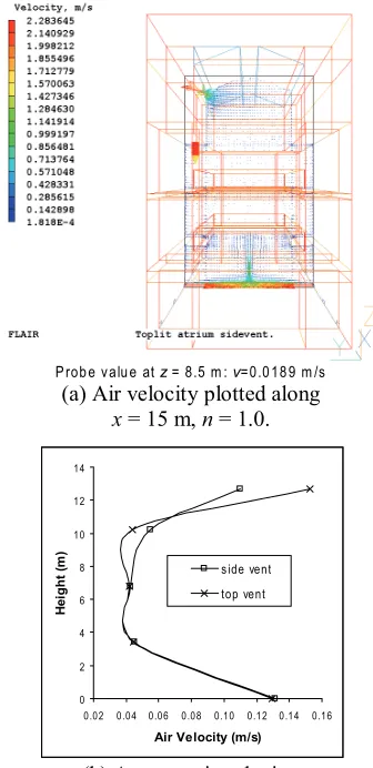
Fig. 8 Air velocity vector plot for model with vertical side vent and average air velocity due
to different outlet’s arrangement.
5. CONCLUSION
This paper has presented a steady-state 3-D CF3-D modelling of air movement and temperature distribution due to thermal buoyancy within top-lit representative Malaysian atrium models with the
ground floor atrium only pressurised
ventilation.
Probe value at z = 8.5 m : v=0.0189 m /s
(a) Air velocity plotted along
x = 15 m, n = 1.0.
0 2 4 6 8 10 12 14
0.02 0.04 0.06 0.08 0.10 0.12 0.14 0.16 Air Velocity (m/s)
He
ig
ht
(m
)
side vent top vent
41
International Journal of Integrated Engineering (Issue on Civil and Environmental Engineering)
Modelling studies investigating the effect of area ratio on the atrium’s thermal performance have revealed that
smaller opening area ratios (i.e. n≤1)
resulted in higher neutral pressure plane level. Higher position of neutral pressure plane level would decrease the pressure difference across the outlet causing lower outlet’s velocity. The consequence was the ventilation capacity at the outlet would also be reduced. As the ventilation capacity at the inlet was constant, higher neutral pressure plane level resulted in the higher inlets’ velocity due to the increase in the pressure difference across the inlet. Hence, the hot indoor air was well-mixed and became rather stagnant as the ventilation capacity at the outlet was low. As such, this would not help improve the thermal conditions particularly on occupied levels.
On the contrary, the thermal conditions, particularly on the occupied levels,
improved considerably with sufficiently
higher opening area ratios (i.e. n>1). This
was due to the fact that sufficiently low
neutral pressure plane level would result in the increase of pressure difference across the outlet; hence, increase the ventilation capacity at the outlet. Subsequently, this would lead to the lowering of indoor air temperature since the ventilation capacity at the inlet was constant.
Surprisingly, it was also revealed that with equal inlet and outlet area (thus, area ratio equal to 1), changing the outlet’s
arrangement (i.e. location and configuration) was not significantly affected the atrium’s
thermal performance. Apparently the high neutral pressure plane level, which was
generally above the second floor level, was the main reason for the insignificant
changes in the air movement and
temperature distribution within the central atrium, particularly on occupied levels. Therefore, in order to better investigate the effect of outlet’s arrangement (i.e. location
and configuration) on the atrium’s thermal
performance particularly within occupied levels, it is recommended for future study to use an area ratio which can result in
sufficiently low neutral pressure plane level
(i.e. generally n>1).
ACKNOWLEDGMENT
This work was carried out as part of the PhD research project funded by the Ministry of Higher Education Malaysia and Universiti Tun Hussein Onn Malaysia. We are particularly grateful to the staff at the School of the Built Environment, Heriot-Watt University, United Kingdom especially Dr Iain MacDougall and Ms Margaret Inglis for providing assistance and technical support during the course of running the simulations.
REFERENCES
[1] A.A. Setrakian and D.A. Morgan, Application of Computational Fluid Dynamics in Building Services Engineering. Computational Fluid Dynamics for the Environmental and Building Services Engineer – Tool or Toy? Seminar organised by the Environmental Engineering Group of the Institution of Mechanical Engineers and held at the Institution of Mechanical Engineers on 26 November 1991. [2] H.K. Versteeg and W. Malalasekera,.
Harlow: Longman Scientific and
Technical, 1995.
[3] Sabarinah, S.A., A Review on Interior
Comfort Conditions in Malaysia. ANZAScA Conference 2002. The
University of Queensland, Brisbane,
Australia, 2002.
[4] P.O. Fanger, Thermal Comfort. Danish Technical Press, Coopenhagen, 1970. [5] ISO 7730, Moderate Thermal
Environments – Determination of the
PMV and PPD Indices and Specification
of the Conditions for Thermal Comfort. 2nd Edition. International Organisation
for Standardization, Geneva,
Switzerland, 1994.
[6] O.H. Koenigsberger, T.G. Ingersoll, A.
Mayhew and S.V. Szokolay, Manual
of Tropical Housing and Building, Part 1: Climatic Design. First Edition. London: Longman, 1980.
[7] K. Takahashi and H. Arakawa, Climate of Southern and West Asia. World Survey of Climatology. 9:1981: pp.62-66, 1981.
[8] S. Nieuwolt, Tropical Climatology: An Introduction to the Climate of the Low Latitudes. London: John Wiley and Sons, 1977.
[9] K.T. Andersen, Natural Ventilation in
Atria. ASHRAE Atrium Symposium,
ASHRAE Technical Data Bulletin. 11(3): 30-38, 1995.
[10] K.T. Andersen, Theory for Natural Ventilation by Thermal Buoyancy in One Zone with Uniform Temperature. Building and Environment. 38: 1281-1289, 2003.
[11] IEA-ECB Annex 26. Energy Efficient
Ventilation of Large Enclosures. IEA – Energy Conservation in Buildings and Community Systems. (P. Heiselberg, S. Murakami and CA editors), 1998.
[12] J.M. Holford and G.R. Hunt,
Fundamental Atrium Design for Natural Ventilation. Building and Environment. 38: 409-426, 2003. [13] F.H. Harlow and P.I. Nakayama,
Turbulent Transport Equation. Phys. Fluids. 10: 2323-332, 1967.
[14] B.E. Launder and D.B. Spalding, Mathematical Models of Turbulence. London: Academic Press, 1972. [15] P.V. Nielsen, Prediction of Temperature
and Velocity Distribution in an
Air-conditioned Room. Proceedings of
the Second Symposium on the Use of Computers for Environmental Engineering Related to Building, Paris, 1974.
[16] Y. Sakamoto and Y.Matsuo, Numerical Predictions of Three-dimensional Flow
in a Ventilated Room using Turbulence
Models. Appl. Math. Modelling. 4: 67-72, 1980.
[17] S. Murakami, S. Kato and Y. Suyama, Three-dimensional Numerical
Simulation of Turbulent Airflow in Ventilated Room by means of
43
International Journal of Integrated Engineering (Issue on Civil and Environmental Engineering)
Analysis and Development of the
Generic Maintenance Management
Process Modeling for the Preservation
of Heritage School Buildings
A Z. A. Akasah1, * and B. M. Alias2
1Faculty of Civil and Enviromental Engineering, Universiti Tun Hussein Onn Malaysia, Malaysia
2Faculty of Technical Education, Universiti Tun Hussein Onn Malaysia, Malaysia *Corresponding email: [email protected]
Abstract
Preservation of heritage school buildings requires special maintenance management practices. A thorough understanding of the maintenance management process is essential in ensuring effective maintenance practices can be instituted. The aim of this paper was to develop a generic process model that will promote the understanding of an effective management of maintenance process for heritage school buildings. A process model for the Maintenance Management of Heritage School Buildings (MMHSB) was developed using the
Integration Definition for Function Modeling (IDEF0) system through an iterative process.
The initial MMHSB process model was submitted to a team of management experts from the Malaysian Ministry of Arts and Heritage and the Ministry of Education Malaysia for
verifications. Based on their feedbacks the initial model was refined and a proposed model was developed. From the second verification, the feed back received formed the basis for the final model. The final model elucidates the items for the input, mechanism, control
and output elements that are critical in the maintenance management of heritage school
buildings. The model also redefines the existing scope of responsibilities of the Headmasters’ and Senior Assistants’ in the management of maintenance. The perceived effectiveness of
the model by potential users was surveyed using a selected number of administrators from potentially recognized heritage schools. The results indicated that the process model is perceived as being helpful in clarifying the maintenance management process of heritage school buildings and is useful in changing the current reactive management practices to that of a more proactive practice. In conclusion, it is believed that the MMHSB Process Model is helpful in promoting the understanding of the maintenance management process which would lead to improve preservation practices of heritage school buildings.