Learning statistics with R:
A tutorial for psychology students and other beginners
(Version 0.6)
Danielle Navarro
University of New South Wales
[email protected]
Overview.
This book is published under a Creative Commons BY-SA license (CC BY-SA) version 4.0. This means that this book can be reused, remixed, retained, revised and redistributed (including commercially) as
long as appropriate credit is given to the authors. If you remix, or modify the original version of this open textbook, you must redistribute all versions of this open textbook under the same license - CC
BY-SA.
Table of Contents
Preface ix
I
Background
1
1 Why do we learn statistics? 3
1.1 On the psychology of statistics . . . 3
1.2 The cautionary tale of Simpson’s paradox . . . 6
1.3 Statistics in psychology . . . 8
1.4 Statistics in everyday life . . . 10
1.5 There’s more to research methods than statistics . . . 10
2 A brief introduction to research design 11 2.1 Introduction to psychological measurement . . . 11
2.2 Scales of measurement . . . 14
2.3 Assessing the reliability of a measurement . . . 19
2.4 The “role” of variables: predictors and outcomes . . . 20
2.5 Experimental and non-experimental research . . . 20
2.6 Assessing the validity of a study . . . 22
2.7 Confounds, artifacts and other threats to validity . . . 25
2.8 Summary. . . 33
II
An introduction to
R
35
3 Getting started withR 37 3.1 InstallingR . . . 383.2 Typing commands at theRconsole . . . 42
3.3 Doing simple calculations withR . . . 46
3.4 Storing a number as a variable . . . 48
3.5 Using functions to do calculations . . . 51
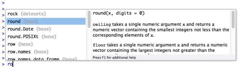
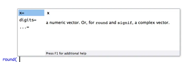
3.6 Letting Rstudio help you with your commands. . . 54
3.7 Storing many numbers as a vector . . . 57
3.8 Storing text data . . . 60
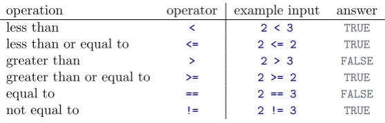
3.9 Storing “true or false” data . . . 61
3.10 Indexing vectors . . . 66
3.11 QuittingR . . . 69
3.12 Summary. . . 70
4 AdditionalRconcepts 73 4.1 Using comments . . . 73
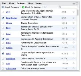
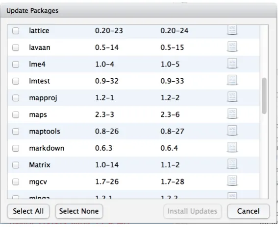
4.2 Installing and loading packages . . . 74
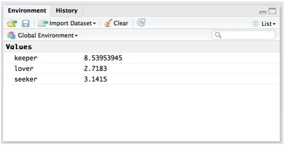
4.3 Managing the workspace . . . 80
4.4 Navigating the file system . . . 83
4.5 Loading and saving data . . . 87
4.6 Useful things to know about variables . . . 93
4.7 Factors . . . 97
4.9 Lists . . . 102
4.10 Formulas . . . 103
4.11 Generic functions . . . 104
4.12 Getting help . . . 105
4.13 Summary. . . 109
III
Working with data
111
5 Descriptive statistics 113 5.1 Measures of central tendency . . . 1145.2 Measures of variability . . . 123
5.3 Skew and kurtosis . . . 131
5.4 Getting an overall summary of a variable . . . 133
5.5 Descriptive statistics separately for each group . . . 136
5.6 Standard scores . . . 138
5.7 Correlations . . . 139
5.8 Handling missing values . . . 151
5.9 Summary. . . 154
6 Drawing graphs 157 6.1 An overview of Rgraphics . . . 158
6.2 An introduction to plotting . . . 160
6.3 Histograms. . . 170
6.4 Stem and leaf plots . . . 173
6.5 Boxplots . . . 175
6.6 Scatterplots . . . 183
6.7 Bar graphs . . . 187
6.8 Saving image files usingRand Rstudio . . . 191
6.9 Summary. . . 193
7 Pragmatic matters 195 7.1 Tabulating and cross-tabulating data . . . 196
7.2 Transforming and recoding a variable . . . 199
7.3 A few more mathematical functions and operations . . . 203
7.4 Extracting a subset of a vector . . . 207
7.5 Extracting a subset of a data frame . . . 210
7.6 Sorting, flipping and merging data . . . 218
7.7 Reshaping a data frame. . . 224
7.8 Working with text . . . 229
7.9 Reading unusual data files . . . 237
7.10 Coercing data from one class to another . . . 241
7.11 Other useful data structures . . . 242
7.12 Miscellaneous topics . . . 247
7.13 Summary. . . 252
8 Basic programming 253 8.1 Scripts . . . 253
8.2 Loops. . . 259
8.3 Conditional statements . . . 263
8.4 Writing functions . . . 264
8.6 Summary. . . 268
IV
Statistical theory
269
9 Introduction to probability 275 9.1 How are probability and statistics different? . . . 2769.2 What does probability mean? . . . 277
9.3 Basic probability theory . . . 281
9.4 The binomial distribution . . . 283
9.5 The normal distribution . . . 289
9.6 Other useful distributions . . . 294
9.7 Summary. . . 298
10 Estimating unknown quantities from a sample 301 10.1 Samples, populations and sampling . . . 301
10.2 The law of large numbers . . . 308
10.3 Sampling distributions and the central limit theorem . . . 309
10.4 Estimating population parameters . . . 315
10.5 Estimating a confidence interval . . . 320
10.6 Summary. . . 326
11 Hypothesis testing 327 11.1 A menagerie of hypotheses . . . 327
11.2 Two types of errors . . . 330
11.3 Test statistics and sampling distributions . . . 332
11.4 Making decisions . . . 333
11.5 Thepvalue of a test . . . 336
11.6 Reporting the results of a hypothesis test . . . 338
11.7 Running the hypothesis test in practice . . . 340
11.8 Effect size, sample size and power . . . 341
11.9 Some issues to consider . . . 346
11.10 Summary. . . 348
V
Statistical tools
349
12 Categorical data analysis 351 12.1 Theχ2goodness-of-fit test . . . 35112.2 Theχ2test of independence (or association) . . . 363
12.3 The continuity correction . . . 369
12.4 Effect size . . . 370
12.5 Assumptions of the test(s) . . . 371
12.6 The most typical way to do chi-square tests inR. . . 371
12.7 The Fisher exact test . . . 373
12.8 The McNemar test . . . 375
12.9 What’s the difference between McNemar and independence? . . . 377
13 Comparing two means 379
13.1 The one-samplez-test. . . 379
13.2 The one-samplet-test . . . 385
13.3 The independent samplest-test (Student test) . . . 389
13.4 The independent samplest-test (Welch test) . . . 398
13.5 The paired-samplest-test . . . 400
13.6 One sided tests . . . 408
13.7 Using the t.test() function . . . 410
13.8 Effect size . . . 412
13.9 Checking the normality of a sample . . . 416
13.10 Testing non-normal data with Wilcoxon tests . . . 420
13.11 Summary. . . 422
14 Comparing several means (one-way ANOVA) 425 14.1 An illustrative data set . . . 425
14.2 How ANOVA works . . . 427
14.3 Running an ANOVA inR. . . 437
14.4 Effect size . . . 440
14.5 Multiple comparisons and post hoc tests . . . 441
14.6 Assumptions of one-way ANOVA . . . 446
14.7 Checking the homogeneity of variance assumption . . . 447
14.8 Removing the homogeneity of variance assumption . . . 449
14.9 Checking the normality assumption . . . 450
14.10 Removing the normality assumption . . . 450
14.11 On the relationship between ANOVA and the Studentttest . . . 453
14.12 Summary. . . 454
15 Linear regression 457 15.1 What is a linear regression model? . . . 457
15.2 Estimating a linear regression model . . . 459
15.3 Multiple linear regression . . . 461
15.4 Quantifying the fit of the regression model . . . 464
15.5 Hypothesis tests for regression models . . . 466
15.6 Testing the significance of a correlation . . . 470
15.7 Regarding regression coefficients . . . 472
15.8 Assumptions of regression . . . 474
15.9 Model checking . . . 475
15.10 Model selection . . . 490
15.11 Summary. . . 495
16 Factorial ANOVA 497 16.1 Factorial ANOVA 1: balanced designs, no interactions . . . 497
16.2 Factorial ANOVA 2: balanced designs, interactions allowed. . . 506
16.3 Effect size, estimated means, and confidence intervals . . . 513
16.4 Assumption checking . . . 517
16.5 TheF test as a model comparison. . . 518
16.6 ANOVA as a linear model . . . 521
16.7 Different ways to specify contrasts. . . 532
16.8 Post hoc tests . . . 537
16.9 The method of planned comparisons . . . 539
16.10 Factorial ANOVA 3: unbalanced designs . . . 539
VI
Endings, alternatives and prospects
553
17 Bayesian statistics 555
17.1 Probabilistic reasoning by rational agents. . . 555
17.2 Bayesian hypothesis tests . . . 560
17.3 Why be a Bayesian? . . . 562
17.4 Bayesian analysis of contingency tables . . . 568
17.5 Bayesiant-tests . . . 574
17.6 Bayesian regression . . . 577
17.7 Bayesian ANOVA . . . 581
17.8 Summary. . . 584
18 Epilogue 587 18.1 The undiscovered statistics . . . 587
18.2 Learning the basics, and learning them inR . . . 595
Preface to Version 0.6
The book hasn’t changed much since 2015 when I released Version 0.5 – it’s probably fair to say that I’ve changed more than it has. I moved from Adelaide to Sydney in 2016 and my teaching profile at UNSW is different to what it was at Adelaide, and I haven’t really had a chance to work on it since arriving here! It’s a little strange looking back at this actually. A few quick comments...
• Weirdly, the bookconsistentlymisgenders me, but I suppose I have only myself to blame for that one :-) There’s now a brief footnote on page 12 that mentions this issue; in real life I’ve been working through a gender affirmation process for the last two years and mostly go by she/her pronouns. I am, however, just as lazy as I ever was so I haven’t bothered updating the text in the book.
• For Version 0.6 I haven’t changed much I’ve made a few minor changes when people have pointed out typos or other errors. In particular it’s worth noting the issue associated with the etaSquared function in thelsr package (which isn’t really being maintained any more) in Section 14.4. The function works fine for the simple examples in the book, but there are definitely bugs in there that I haven’t found time to check! So please take care with that one.
• The biggest change really is the licensing! I’ve released it under a Creative Commons licence (CC BY-SA 4.0, specifically), and placed all the source files to the associated GitHub repository, if anyone wants to adapt it.
Maybe someone would like to write a version that makes use of the tidyverse... I hear that’s become rather important to R these days :-)
Best,
Danielle Navarro
Preface to Version 0.5
Another year, another update. This time around, the update has focused almost entirely on the theory sections of the book. Chapters 9, 10 and 11 have been rewritten, hopefully for the better. Along the same lines, Chapter 17 is entirely new, and focuses on Bayesian statistics. I think the changes have improved the book a great deal. I’ve always felt uncomfortable about the fact that all the inferential statistics in the book are presented from an orthodox perspective, even though I almost always present Bayesian data analyses in my own work. Now that I’ve managed to squeeze Bayesian methods into the book somewhere, I’m starting to feel better about the book as a whole. I wanted to get a few other things done in this update, but as usual I’m running into teaching deadlines, so the update has to go out the way it is!
February 16, 2015
Preface to Version 0.4
A year has gone by since I wrote the last preface. The book has changed in a few important ways: Chapters 3 and 4 do a better job of documenting some of the time saving features of Rstudio, Chapters 12 and 13 now make use of new functions in the lsr package for running chi-square tests and t tests, and the discussion of correlations has been adapted to refer to the new functions in the lsr package. The soft copy of 0.4 now has better internal referencing (i.e., actual hyperlinks between sections), though that was introduced in 0.3.1. There’s a few tweaks here and there, and many typo corrections (thank you to everyone who pointed out typos!), but overall 0.4 isn’t massively different from 0.3.
I wish I’d had more time over the last 12 months to add more content. The absence of any discussion of repeated measures ANOVA and mixed models more generally really does annoy me. My excuse for this lack of progress is that my second child was born at the start of 2013, and so I spent most of last year just trying to keep my head above water. As a consequence, unpaid side projects like this book got sidelined in favour of things that actually pay my salary! Things are a little calmer now, so with any luck version 0.5 will be a bigger step forward.
One thing that has surprised me is the number of downloads the book gets. I finally got some basic tracking information from the website a couple of months ago, and (after excluding obvious robots) the book has been averaging about 90 downloads per day. That’s encouraging: there’s at least a few people who find the book useful!
Preface to Version 0.3
There’s a part of me that really doesn’t want to publish this book. It’s not finished.
And when I say that, I mean it. The referencing is spotty at best, the chapter summaries are just lists of section titles, there’s no index, there are no exercises for the reader, the organisation is suboptimal, and the coverage of topics is just not comprehensive enough for my liking. Additionally, there are sections with content that I’m not happy with, figures that really need to be redrawn, and I’ve had almost no time to hunt down inconsistencies, typos, or errors. In other words, this book is not finished. If I didn’t have a looming teaching deadline and a baby due in a few weeks, I really wouldn’t be making this available at all.
What this means is that if you are an academic looking for teaching materials, a Ph.D. student looking to learnR, or just a member of the general public interested in statistics, I would advise you to be cautious. What you’re looking at is a first draft, and it may not serve your purposes. If we were living in the days when publishing was expensive and the internet wasn’t around, I would never consider releasing a book in this form. The thought of someong shelling out $80 for this (which is what a commercial publisher told me it would retail for when they offered to distribute it) makes me feel more than a little uncomfortable. However, it’s the 21st century, so I can post the pdf on my website for free, and I can distribute hard copies via a print-on-demand service for less than half what a textbook publisher would charge. And so my guilt is assuaged, and I’m willing to share! With that in mind, you can obtain free soft copies and cheap hard copies online, from the following webpages:
Soft copy: http://www.compcogscisydney.com/learning-statistics-with-r.html
Hard copy: www.lulu.com/content/13570633
Even so, the warning still stands: what you are looking at is Version 0.3 of a work in progress. If and when it hits Version 1.0, I would be willing to stand behind the work and say, yes, this is a textbook that I would encourage other people to use. At that point, I’ll probably start shamelessly flogging the thing on the internet and generally acting like a tool. But until that day comes, I’d like it to be made clear that I’m really ambivalent about the work as it stands.
All of the above being said, there is one group of people that I can enthusiastically endorse this book to: the psychology students taking our undergraduate research methods classes (DRIP and DRIP:A) in 2013. For you, this book is ideal, because it was written to accompany your stats lectures. If a problem arises due to a shortcoming of these notes, I can and will adapt content on the fly to fix that problem. Effectively, you’ve got a textbook written specifically for your classes, distributed for free (electronic copy) or at near-cost prices (hard copy). Better yet, the notes have been tested: Version 0.1 of these notes was used in the 2011 class, Version 0.2 was used in the 2012 class, and now you’re looking at the new and improved Version 0.3. I’m not saying these notes are titanium plated awesomeness on a stick – though ifyouwanted to say so on the student evaluation forms, then you’re totally welcome to – because they’re not. But I am saying that they’ve been tried out in previous years and they seem to work okay. Besides, there’s a group of us around to troubleshoot if any problems come up, and you can guarantee that at leastoneof your lecturers has read the whole thing cover to cover!
and density is discussed. A detailed treatment of Type I, II and III sums of squares for unbalanced factorial ANOVA is provided. And if you have a look in the Epilogue, it should be clear that my intention is to add a lot more advanced content.
My reasons for pursuing this approach are pretty simple: the students can handle it, and they even seem to enjoy it. Over the last few years I’ve been pleasantly surprised at just how little difficulty I’ve had in getting undergraduate psych students to learnR. It’s certainly not easy for them, and I’ve found I need to be a little charitable in setting marking standards, but they do eventually get there. Similarly, they don’t seem to have a lot of problems tolerating ambiguity and complexity in presentation of statistical ideas, as long as they are assured that the assessment standards will be set in a fashion that is appropriate for them. So if the students can handle it, why not teach it? The potential gains are pretty enticing. If they learnR, the students get access to CRAN, which is perhaps the largest and most comprehensive library of statistical tools in existence. And if they learn about probability theory in detail, it’s easier for them to switch from orthodox null hypothesis testing to Bayesian methods if they want to. Better yet, they learn data analysis skills that they can take to an employer without being dependent on expensive and proprietary software.
Sadly, this book isn’t the silver bullet that makes all this possible. It’s a work in progress, and maybe when it is finished it will be a useful tool. One among many, I would think. There are a number of other books that try to provide a basic introduction to statistics using R, and I’m not arrogant enough to believe that mine is better. Still, I rather like the book, and maybe other people will find it useful, incomplete though it is.
Part I.
1. Why do we learn statistics?
“Thou shalt not answer questionnaires Or quizzes upon World Affairs,
Nor with compliance
Take any test. Thou shalt not sit With statisticians nor commit
A social science”
– W.H. Auden1
1.1
On the psychology of statistics
To the surprise of many students, statistics is a fairly significant part of a psychological education. To the surprise of no-one, statistics is very rarely the favouritepart of one’s psychological education. After all, if you really loved the idea of doing statistics, you’d probably be enrolled in a statistics class right now, not a psychology class. So, not surprisingly, there’s a pretty large proportion of the student base that isn’t happy about the fact that psychology has so much statistics in it. In view of this, I thought that the right place to start might be to answer some of the more common questions that people have about stats. . .
A big part of this issue at hand relates to the very idea of statistics. What is it? What’s it there for? And why are scientists so bloody obsessed with it? These are all good questions, when you think about it. So let’s start with the last one. As a group, scientists seem to be bizarrely fixated on running statistical tests on everything. In fact, we use statistics so often that we sometimes forget to explain to people why we do. It’s a kind of article of faith among scientists – and especially social scientists – that your findings can’t be trusted until you’ve done some stats. Undergraduate students might be forgiven for thinking that we’re all completely mad, because no-one takes the time to answer one very simple question:
Why do you do statistics? Why don’t scientists just use common sense?
It’s a naive question in some ways, but most good questions are. There’s a lot of good answers to it,2
1The quote comes from Auden’s 1946 poemUnder Which Lyre: A Reactionary Tract for the Times, delivered as part of
a commencement address at Harvard University. The history of the poem is kind of interesting: http://harvardmagazine .com/2007/11/a-poets-warning.html
but for my money, the best answer is a really simple one: we don’t trust ourselves enough. We worry that we’re human, and susceptible to all of the biases, temptations and frailties that humans suffer from. Much of statistics is basically a safeguard. Using “common sense” to evaluate evidence means trusting gut instincts, relying on verbal arguments and on using the raw power of human reason to come up with the right answer. Most scientists don’t think this approach is likely to work.
In fact, come to think of it, this sounds a lot like a psychological question to me, and since I do work in a psychology department, it seems like a good idea to dig a little deeper here. Is it really plausible to think that this “common sense” approach is very trustworthy? Verbal arguments have to be constructed in language, and all languages have biases – some things are harder to say than others, and not necessarily because they’re false (e.g., quantum electrodynamics is a good theory, but hard to explain in words). The instincts of our “gut” aren’t designed to solve scientific problems, they’re designed to handle day to day inferences – and given that biological evolution is slower than cultural change, we should say that they’re designed to solve the day to day problems for a different world than the one we live in. Most fundamentally, reasoning sensibly requires people to engage in “induction”, making wise guesses and going beyond the immediate evidence of the senses to make generalisations about the world. If you think that you can do that without being influenced by various distractors, well, I have a bridge in Brooklyn I’d like to sell you. Heck, as the next section shows, we can’t even solve “deductive” problems (ones where no guessing is required) without being influenced by our pre-existing biases.
1.1.1
The curse of belief bias
People are mostly pretty smart. We’re certainly smarter than the other species that we share the planet with (though many people might disagree). Our minds are quite amazing things, and we seem to be capable of the most incredible feats of thought and reason. That doesn’t make us perfect though. And among the many things that psychologists have shown over the years is that we really do find it hard to be neutral, to evaluate evidence impartially and without being swayed by pre-existing biases. A good example of this is thebelief bias effectin logical reasoning: if you ask people to decide whether a particular argument is logically valid (i.e., conclusion would be true if the premises were true), we tend to be influenced by the believability of the conclusion, even when we shouldn’t. For instance, here’s a valid argument where the conclusion is believable:
No cigarettes are inexpensive (Premise 1)
Some addictive things are inexpensive (Premise 2)
Therefore, some addictive things are not cigarettes (Conclusion)
And here’s a valid argument where the conclusion is not believable:
No addictive things are inexpensive (Premise 1) Some cigarettes are inexpensive (Premise 2)
Therefore, some cigarettes are not addictive (Conclusion)
The logicalstructureof argument #2 is identical to the structure of argument #1, and they’re both valid. However, in the second argument, there are good reasons to think that premise 1 is incorrect, and as a result it’s probably the case that the conclusion is also incorrect. But that’s entirely irrelevant to the topic at hand: an argument is deductively valid if the conclusion is a logical consequence of the premises. That is, a valid argument doesn’t have to involve true statements.
On the other hand, here’s an invalid argument that has a believable conclusion:
No addictive things are inexpensive (Premise 1) Some cigarettes are inexpensive (Premise 2)
And finally, an invalid argument with an unbelievable conclusion:
No cigarettes are inexpensive (Premise 1)
Some addictive things are inexpensive (Premise 2) Therefore, some cigarettes are not addictive (Conclusion)
Now, suppose that people really are perfectly able to set aside their pre-existing biases about what is true and what isn’t, and purely evaluate an argument on its logical merits. We’d expect 100% of people to say that the valid arguments are valid, and 0% of people to say that the invalid arguments are valid. So if you ran an experiment looking at this, you’d expect to see data like this:
conclusion feels true conclusion feels false
argument is valid 100% say “valid” 100% say “valid”
argument is invalid 0% say “valid” 0% say “valid”
If the psychological data looked like this (or even a good approximation to this), we might feel safe in just trusting our gut instincts. That is, it’d be perfectly okay just to let scientists evaluate data based on their common sense, and not bother with all this murky statistics stuff. However, you guys have taken psych classes, and by now you probably know where this is going . . .
In a classic study,J. S. B. T. Evans, Barston, and Pollard(1983) ran an experiment looking at exactly this. What they found is that when pre-existing biases (i.e., beliefs) were in agreement with the structure of the data, everything went the way you’d hope:
conclusion feels true conclusion feels false
argument is valid 92% say “valid”
argument is invalid 8% say “valid”
Not perfect, but that’s pretty good. But look what happens when our intuitive feelings about the truth of the conclusion run against the logical structure of the argument:
conclusion feels true conclusion feels false
argument is valid 92% say “valid” 46% say “valid” argument is invalid 92% say “valid” 8% say “valid”
Oh dear, that’s not as good. Apparently, when people are presented with a strong argument that contradicts our pre-existing beliefs, we find it pretty hard to even perceive it to be a strong argument (people only did so 46% of the time). Even worse, when people are presented with a weak argument that agrees with our pre-existing biases, almost no-one can see that the argument is weak (people got that one wrong 92% of the time!)3
If you think about it, it’s not as if these data are horribly damning. Overall, people did do better than chance at compensating for their prior biases, since about 60% of people’s judgements were correct (you’d expect 50% by chance). Even so, if you were a professional “evaluator of evidence”, and someone came along and offered you a magic tool that improves your chances of making the right decision from 60% to (say) 95%, you’d probably jump at it, right? Of course you would. Thankfully, we actually do have a tool that can do this. But it’s not magic, it’s statistics. So that’s reason #1 why scientists love
statistics. It’s justtoo easyfor us to “believe what we want to believe”; so if we want to “believe in the data” instead, we’re going to need a bit of help to keep our personal biases under control. That’s what statistics does: it helps keep us honest.
1.2
The cautionary tale of Simpson’s paradox
The following is a true story (I think...). In 1973, the University of California, Berkeley had some worries about the admissions of students into their postgraduate courses. Specifically, the thing that caused the problem was that the gender breakdown of their admissions, which looked like this. . .
Number of applicants Percent admitted
Males 8442 44%
Females 4321 35%
. . . and the were worried about being sued.4 Given that there were nearly 13,000 applicants, a difference of 9% in admission rates between males and females is just way too big to be a coincidence. Pretty compelling data, right? And if I were to say to you that these dataactuallyreflect a weak bias in favour of women (sort of!), you’d probably think that I was either crazy or sexist.
Oddly, it’s actually sort of true . . . when people started looking more carefully at the admissions data (Bickel, Hammel, & O’Connell, 1975) they told a rather different story. Specifically, when they looked at it on a department by department basis, it turned out that most of the departments actually had a slightly highersuccess rate for female applicants than for male applicants. The table below shows the admission figures for the six largest departments (with the names of the departments removed for privacy reasons):
Males Females
Department Applicants Percent admitted Applicants Percent admitted
A 825 62% 108 82%
B 560 63% 25 68%
C 325 37% 593 34%
D 417 33% 375 35%
E 191 28% 393 24%
F 272 6% 341 7%
Remarkably, most departments had ahigherrate of admissions for females than for males! Yet the overall rate of admission across the university for females waslowerthan for males. How can this be? How can both of these statements be true at the same time?
Here’s what’s going on. Firstly, notice that the departments arenotequal to one another in terms of their admission percentages: some departments (e.g., engineering, chemistry) tended to admit a high per-centage of the qualified applicants, whereas others (e.g., English) tended to reject most of the candidates, even if they were high quality. So, among the six departments shown above, notice that department A is the most generous, followed by B, C, D, E and F in that order. Next, notice that males and females tended to apply to different departments. If we rank the departments in terms of the total number of male applicants, we getAąBąDąCąFąE (the “easy” departments are in bold). On the whole, males
0 20 40 60 80 100
0
20
40
60
80
100
Percentage of female applicants
Admission r
ate (both genders)
Figure 1.1: The Berkeley 1973 college admissions data. This figure plots the admission rate for the 85 departments that had at least one female applicant, as a function of the percentage of applicants that were female. The plot is a redrawing of Figure 1 fromBickel et al.(1975). Circles plot departments with more than 40 applicants; the area of the circle is proportional to the total number of applicants. The crosses plot department with fewer than 40 applicants.
. . . .
tended to apply to the departments that had high admission rates. Now compare this to how the female applicants distributed themselves. Ranking the departments in terms of the total number of female ap-plicants produces a quite different ordering CąEąDąFąAąB. In other words, what these data seem to be suggesting is that the female applicants tended to apply to “harder” departments. And in fact, if we look at all Figure 1.1 we see that this trend is systematic, and quite striking. This effect is known as Simpson’s paradox. It’s not common, but it does happen in real life, and most people are very surprised by it when they first encounter it, and many people refuse to even believe that it’s real. It is very real. And while there are lots of very subtle statistical lessons buried in there, I want to use it to make a much more important point . . . doing research is hard, and there arelotsof subtle, counterintuitive traps lying in wait for the unwary. That’s reason #2 why scientists love statistics, and why we teach research methods. Because science is hard, and the truth is sometimes cunningly hidden in the nooks and crannies of complicated data.
all this with the concern that Berkeley’s admissions processes might be unfairly biased against female applicants. When we looked at the “aggregated” data, it did seem like the university was discriminating against women, but when we “disaggregate” and looked at the individual behaviour of all the depart-ments, it turned out that the actual departments were, if anything, slightly biased in favour of women. The gender bias in total admissions was caused by the fact that women tended to self-select for harder departments. From a legal perspective, that would probably put the university in the clear. Postgraduate admissions are determined at the level of the individual department (and there are good reasons to do that), and at the level of individual departments, the decisions are more or less unbiased (the weak bias in favour of females at that level is small, and not consistent across departments). Since the university can’t dictate which departments people choose to apply to, and the decision making takes place at the level of the department it can hardly be held accountable for any biases that those choices produce.
That was the basis for my somewhat glib remarks earlier, but that’s not exactly the whole story, is it? After all, if we’re interested in this from a more sociological and psychological perspective, we might want to askwhythere are such strong gender differences in applications. Why do males tend to apply to engineering more often than females, and why is this reversed for the English department? And why is it it the case that the departments that tend to have a female-application bias tend to have lower overall admission rates than those departments that have a male-application bias? Might this not still reflect a gender bias, even though every single department is itself unbiased? It might. Suppose, hypothetically, that males preferred to apply to “hard sciences” and females prefer “humanities”. And suppose further that the reason for why the humanities departments have low admission rates is because the government doesn’t want to fund the humanities (Ph.D. places, for instance, are often tied to government funded research projects). Does that constitute a gender bias? Or just an unenlightened view of the value of the humanities? What if someone at a high level in the government cut the humanities funds because they felt that the humanities are “useless chick stuff”. That seems prettyblatantlygender biased. None of this falls within the purview of statistics, but it matters to the research project. If you’re interested in the overall structural effects of subtle gender biases, then you probably want to look at boththe aggregated and disaggregated data. If you’re interested in the decision making process at Berkeley itself then you’re probably only interested in the disaggregated data.
In short there are a lot of critical questions that you can’t answer with statistics, but the answers to those questions will have a huge impact on how you analyse and interpret data. And this is the reason why you should always think of statistics as a tool to help you learn about your data, no more and no less. It’s a powerful tool to that end, but there’s no substitute for careful thought.
1.3
Statistics in psychology
I hope that the discussion above helped explain why science in general is so focused on statistics. But I’m guessing that you have a lot more questions about what role statistics plays in psychology, and specifically why psychology classes always devote so many lectures to stats. So here’s my attempt to answer a few of them...
• Why does psychology have so much statistics?
experiment, and they don’t get angry at the experimenter and then deliberately try to sabotage the data set (not that I’ve ever done that . . . ). At a fundamental level psychology is harder than physics.5
Basically, we teach statistics to you as psychologists because you need to be better at stats than physicists. There’s actually a saying used sometimes in physics, to the effect that “if your experiment needs statistics, you should have done a better experiment”. They have the luxury of being able to say that because their objects of study are pathetically simple in comparison to the vast mess that confronts social scientists. It’s not just psychology, really: most social sciences are desperately reliant on statistics. Not because we’re bad experimenters, but because we’ve picked a harder problem to solve. We teach you stats because you really, really need it.
• Can’t someone else do the statistics?
To some extent, but not completely. It’s true that you don’t need to become a fully trained statistician just to do psychology, but you do need to reach a certain level of statistical competence. In my view, there’s three reasons that every psychological researcher ought to be able to do basic statistics:
– Firstly, there’s the fundamental reason: statistics is deeply intertwined with research design. If you want to be good at designing psychological studies, you need to at least understand the basics of stats.
– Secondly, if you want to be good at the psychological side of the research, then you need to be able to understand the psychological literature, right? But almost every paper in the psychological literature reports the results of statistical analyses. So if you really want to understand the psychology, you need to be able to understand what other people did with their data. And that means understanding a certain amount of statistics.
– Thirdly, there’s a big practical problem with being dependent on other people to do all your statistics: statistical analysis is expensive. If you ever get bored and want to look up how much the Australian government charges for university fees, you’ll notice something interesting: statistics is designated as a “national priority” category, and so the fees are much, much lower than for any other area of study. This is because there’s a massive shortage of statisticians out there. So, from your perspective as a psychological researcher, the laws of supply and demand aren’t exactly on your side here! As a result, in almost any real life situation where you want to do psychological research, the cruel facts will be that you don’t have enough money to afford a statistician. So the economics of the situation mean that you have to be pretty self-sufficient.
Note that a lot of these reasons generalise beyond researchers. If you want to be a practicing psychologist and stay on top of the field, it helps to be able to read the scientific literature, which relies pretty heavily on statistics.
• I don’t care about jobs, research, or clinical work. Do I need statistics?
Okay, now you’re just messing with me. Still, I think it should matter to you too. Statistics should matter to you in the same way that statistics should matter toeveryone: we live in the 21st century, and data areeverywhere. Frankly, given the world in which we live these days, a basic knowledge of statistics is pretty damn close to a survival tool! Which is the topic of the next section...
1.4
Statistics in everyday life
“We are drowning in information, but we are starved for knowledge”
– Various authors, original probably John Naisbitt
When I started writing up my lecture notes I took the 20 most recent news articles posted to the ABC news website. Of those 20 articles, it turned out that 8 of them involved a discussion of something that I would call a statistical topic; 6 of those made a mistake. The most common error, if you’re curious, was failing to report baseline data (e.g., the article mentions that 5% of people in situation X have some characteristic Y, but doesn’t say how common the characteristic is for everyone else!) The point I’m trying to make here isn’t that journalists are bad at statistics (though they almost always are), it’s that a basic knowledge of statistics is very helpful for trying to figure out when someone else is either making a mistake or even lying to you. In fact, one of the biggest things that a knowledge of statistics does to you is cause you to get angry at the newspaper or the internet on a far more frequent basis: you can find a good example of this in Section5.1.5. In later versions of this book I’ll try to include more anecdotes along those lines.
1.5
There’s more to research methods than statistics
So far, most of what I’ve talked about is statistics, and so you’d be forgiven for thinking that statistics is all I care about in life. To be fair, you wouldn’t be far wrong, but research methodology is a broader concept than statistics. So most research methods courses will cover a lot of topics that relate much more to the pragmatics of research design, and in particular the issues that you encounter when trying to do research with humans. However, about 99% of studentfearsrelate to the statistics part of the course, so I’ve focused on the stats in this discussion, and hopefully I’ve convinced you that statistics matters, and more importantly, that it’s not to be feared. That being said, it’s pretty typical for introductory research methods classes to be very stats-heavy. This is not (usually) because the lecturers are evil people. Quite the contrary, in fact. Introductory classes focus a lot on the statistics because you almost always find yourself needing statistics before you need the other research methods training. Why? Because almost all of your assignments in other classes will rely on statistical training, to a much greater extent than they rely on other methodological tools. It’s not common for undergraduate assignments to require you to design your own study from the ground up (in which case you would need to know a lot about research design), but itiscommon for assignments to ask you to analyse and interpret data that were collected in a study that someone else designed (in which case you need statistics). In that sense, from the perspective of allowing you to do well in all your other classes, the statistics is more urgent.
2. A brief introduction to research design
To consult the statistician after an experiment is finished is often merely to ask him to conduct a post mortem examination. He can perhaps say what the experiment died of.
– Sir Ronald Fisher1
In this chapter, we’re going to start thinking about the basic ideas that go into designing a study, collecting data, checking whether your data collection works, and so on. It won’t give you enough information to allow you to design studies of your own, but it will give you a lot of the basic tools that you need to assess the studies done by other people. However, since the focus of this book is much more on data analysis than on data collection, I’m only giving a very brief overview. Note that this chapter is “special” in two ways. Firstly, it’s much more psychology-specific than the later chapters. Secondly, it focuses much more heavily on the scientific problem of research methodology, and much less on the statistical problem of data analysis. Nevertheless, the two problems are related to one another, so it’s traditional for stats textbooks to discuss the problem in a little detail. This chapter relies heavily on Campbell and Stanley(1963) for the discussion of study design, andStevens(1946) for the discussion of scales of measurement. Later versions will attempt to be more precise in the citations.
2.1
Introduction to psychological measurement
The first thing to understand is data collection can be thought of as a kind of measurement. That is, what we’re trying to do here is measure something about human behaviour or the human mind. What do I mean by “measurement”?
2.1.1
Some thoughts about psychological measurement
Measurement itself is a subtle concept, but basically it comes down to finding some way of assigning numbers, or labels, or some other kind of well-defined descriptions to “stuff”. So, any of the following would count as a psychological measurement:
• Myageis33 years. • Ido notlike anchovies.
1Presidential Address to the First Indian Statistical Congress, 1938. Source:
• Mychromosomal gender ismale. • Myself-identified gender ismale.2
In the short list above, thebolded partis “the thing to be measured”, and theitalicised partis “the measurement itself”. In fact, we can expand on this a little bit, by thinking about the set of possible measurements that could have arisen in each case:
• Myage (in years) could have been0, 1, 2, 3 . . ., etc. The upper bound on what my age could possibly be is a bit fuzzy, but in practice you’d be safe in saying that the largest possible age is 150, since no human has ever lived that long.
• When asked if Ilike anchovies, I might have said thatI do, orI do not, or I have no opinion, or I sometimes do.
• Mychromosomal genderis almost certainly going to be male (XY) orfemale (XX), but there are a few other possibilities. I could also haveKlinfelter’s syndrome (XXY), which is more similar to male than to female. And I imagine there are other possibilities too.
• Myself-identified gender is also very likely to bemale or female, but it doesn’t have to agree with my chromosomal gender. I may also choose to identify withneither, or to explicitly call myself transgender.
As you can see, for some things (like age) it seems fairly obvious what the set of possible measurements should be, whereas for other things it gets a bit tricky. But I want to point out that even in the case of someone’s age, it’s much more subtle than this. For instance, in the example above, I assumed that it was okay to measure age in years. But if you’re a developmental psychologist, that’s way too crude, and so you often measure age inyears and months(if a child is 2 years and 11 months, this is usually written as “2;11”). If you’re interested in newborns, you might want to measure age indays since birth, maybe even hours since birth. In other words, the way in which you specify the allowable measurement values is important.
Looking at this a bit more closely, you might also realise that the concept of “age” isn’t actually all that precise. In general, when we say “age” we implicitly mean “the length of time since birth”. But that’s not always the right way to do it. Suppose you’re interested in how newborn babies control their eye movements. If you’re interested in kids that young, you might also start to worry that “birth” is not the only meaningful point in time to care about. If Baby Alice is born 3 weeks premature and Baby Bianca is born 1 week late, would it really make sense to say that they are the “same age” if we encountered them “2 hours after birth”? In one sense, yes: by social convention, we use birth as our reference point for talking about age in everyday life, since it defines the amount of time the person has been operating as an independent entity in the world, but from a scientific perspective that’s not the only thing we care about. When we think about the biology of human beings, it’s often useful to think of ourselves as organisms that have been growing and maturing since conception, and from that perspective Alice and Bianca aren’t the same age at all. So you might want to define the concept of “age” in two
different ways: the length of time since conception, and the length of time since birth. When dealing with adults, it won’t make much difference, but when dealing with newborns it might.
Moving beyond these issues, there’s the question of methodology. What specific “measurement method” are you going to use to find out someone’s age? As before, there are lots of different possi-bilities:
• You could just ask people “how old are you?” The method of self-report is fast, cheap and easy, but it only works with people old enough to understand the question, and some people lie about their age.
• You could ask an authority (e.g., a parent) “how old is your child?” This method is fast, and when dealing with kids it’s not all that hard since the parent is almost always around. It doesn’t work as well if you want to know “age since conception”, since a lot of parents can’t say for sure when conception took place. For that, you might need a different authority (e.g., an obstetrician).
• You could look up official records, like birth certificates. This is time consuming and annoying, but it has its uses (e.g., if the person is now dead).
2.1.2
Operationalisation: defining your measurement
All of the ideas discussed in the previous section all relate to the concept ofoperationalisation. To be a bit more precise about the idea, operationalisation is the process by which we take a meaningful but somewhat vague concept, and turn it into a precise measurement. The process of operationalisation can involve several different things:
• Being precise about what you are trying to measure. For instance, does “age” mean “time since birth” or “time since conception” in the context of your research?
• Determining what method you will use to measure it. Will you use self-report to measure age, ask a parent, or look up an official record? If you’re using self-report, how will you phrase the question?
• Defining the set of the allowable values that the measurement can take. Note that these values don’t always have to be numerical, though they often are. When measuring age, the values are numerical, but we still need to think carefully about what numbers are allowed. Do we want age in years, years and months, days, hours? Etc. For other types of measurements (e.g., gender), the values aren’t numerical. But, just as before, we need to think about what values are allowed. If we’re asking people to self-report their gender, what options to we allow them to choose between? Is it enough to allow only “male” or “female”? Do you need an “other” option? Or should we not give people any specific options, and let them answer in their own words? And if you open up the set of possible values to include all verbal response, how will you interpret their answers?
Operationalisation is a tricky business, and there’s no “one, true way” to do it. The way in which you choose to operationalise the informal concept of “age” or “gender” into a formal measurement depends on what you need to use the measurement for. Often you’ll find that the community of scientists who work in your area have some fairly well-established ideas for how to go about it. In other words, operationalisation needs to be thought through on a case by case basis. Nevertheless, while there a lot of issues that are specific to each individual research project, there are some aspects to it that are pretty general.
• A theoretical construct. This is the thing that you’re trying to take a measurement of, like “age”, “gender” or an “opinion”. A theoretical construct can’t be directly observed, and often they’re actually a bit vague.
• A measure. The measure refers to the method or the tool that you use to make your observations. A question in a survey, a behavioural observation or a brain scan could all count as a measure.
• An operationalisation. The term “operationalisation” refers to the logical connection between the measure and the theoretical construct, or to the process by which we try to derive a measure from a theoretical construct.
• A variable. Finally, a new term. A variable is what we end up with when we apply our measure to something in the world. That is, variables are the actual “data” that we end up with in our data sets.
In practice, even scientists tend to blur the distinction between these things, but it’s very helpful to try to understand the differences.
2.2
Scales of measurement
As the previous section indicates, the outcome of a psychological measurement is called a variable. But not all variables are of the same qualitative type, and it’s very useful to understand what types there are. A very useful concept for distinguishing between different types of variables is what’s known as scales of measurement.
2.2.1
Nominal scale
Anominal scalevariable (also referred to as acategoricalvariable) is one in which there is no particular relationship between the different possibilities: for these kinds of variables it doesn’t make any sense to say that one of them is “bigger’ or “better” than any other one, and it absolutely doesn’t make any sense to average them. The classic example for this is “eye colour”. Eyes can be blue, green and brown, among other possibilities, but none of them is any “better” than any other one. As a result, it would feel really weird to talk about an “average eye colour”. Similarly, gender is nominal too: male isn’t better or worse than female, neither does it make sense to try to talk about an “average gender”. In short, nominal scale variables are those for which the only thing you can say about the different possibilities is that they are different. That’s it.
that when I ask 100 people how they got to work today, and I get this:
Transportation Number of people
(1) Train 12
(2) Bus 30
(3) Car 48
(4) Bicycle 10
So, what’s the average transportation type? Obviously, the answer here is that there isn’t one. It’s a silly question to ask. You can say that travel by car is the most popular method, and travel by train is the least popular method, but that’s about all. Similarly, notice that the order in which I list the options isn’t very interesting. I could have chosen to display the data like this
Transportation Number of people
(3) Car 48
(1) Train 12
(4) Bicycle 10
(2) Bus 30
and nothing really changes.
2.2.2
Ordinal scale
Ordinal scalevariables have a bit more structure than nominal scale variables, but not by a lot. An ordinal scale variable is one in which there is a natural, meaningful way to order the different possibilities, but you can’t do anything else. The usual example given of an ordinal variable is “finishing position in a race”. Youcan say that the person who finished first was faster than the person who finished second, but youdon’tknow how much faster. As a consequence we know that 1stą2nd, and we know that 2nd ą3rd, but the difference between 1st and 2nd might be much larger than the difference between 2nd and 3rd.
Here’s an more psychologically interesting example. Suppose I’m interested in people’s attitudes to climate change, and I ask them to pick one of these four statements that most closely matches their beliefs:
(1) Temperatures are rising, because of human activity (2) Temperatures are rising, but we don’t know why (3) Temperatures are rising, but not because of humans (4) Temperatures are not rising
Notice that these four statements actually do have a natural ordering, in terms of “the extent to which they agree with the current science”. Statement 1 is a close match, statement 2 is a reasonable match, statement 3 isn’t a very good match, and statement 4 is in strong opposition to the science. So, in terms of the thing I’m interested in (the extent to which people endorse the science), I can order the items as 1ą2ą3ą4. Since this ordering exists, it would be very weird to list the options like this. . .
(3) Temperatures are rising, but not because of humans (1) Temperatures are rising, because of human activity (4) Temperatures are not rising
(2) Temperatures are rising, but we don’t know why
So, let’s suppose I asked 100 people these questions, and got the following answers:
Response Number
(1) Temperatures are rising, because of human activity 51 (2) Temperatures are rising, but we don’t know why 20 (3) Temperatures are rising, but not because of humans 10
(4) Temperatures are not rising 19
When analysing these data, it seems quite reasonable to try to group (1), (2) and (3) together, and say that 81 of 100 people were willing toat least partiallyendorse the science. And it’salsoquite reasonable to group (2), (3) and (4) together and say that 49 of 100 people registered at least some disagreement with the dominant scientific view. However, it would be entirely bizarre to try to group (1), (2) and (4) together and say that 90 of 100 people said. . . what? There’s nothing sensible that allows you to group those responses together at all.
That said, notice that while we can use the natural ordering of these items to construct sensible groupings, what we can’t do is average them. For instance, in my simple example here, the “average” response to the question is 1.97. If you can tell me what that means, I’d love to know. Because that sounds like gibberish to me!
2.2.3
Interval scale
In contrast to nominal and ordinal scale variables,interval scaleand ratio scale variables are vari-ables for which the numerical value is genuinely meaningful. In the case of interval scale varivari-ables, the differences between the numbers are interpretable, but the variable doesn’t have a “natural” zero value. A good example of an interval scale variable is measuring temperature in degrees celsius. For instance, if it was 15˝ yesterday and 18˝ today, then the 3˝ difference between the two is genuinely meaningful.
Moreover, that 3˝difference isexactly the sameas the 3˝difference between 7˝and 10˝. In short, addition
and subtraction are meaningful for interval scale variables.3
However, notice that the 0˝does not mean “no temperature at all”: it actually means “the temperature
at which water freezes”, which is pretty arbitrary. As a consequence, it becomes pointless to try to multiply and divide temperatures. It is wrong to say that 20˝ is twice as hotas 10˝, just as it is weird
and meaningless to try to claim that 20˝ is negative two times as hot as´10˝.
Again, lets look at a more psychological example. Suppose I’m interested in looking at how the attitudes of first-year university students have changed over time. Obviously, I’m going to want to record the year in which each student started. This is an interval scale variable. A student who started in 2003 did arrive 5 years before a student who started in 2008. However, it would be completely insane for me to divide 2008 by 2003 and say that the second student started “1.0024 times later” than the first one. That doesn’t make any sense at all.
2.2.4
Ratio scale
The fourth and final type of variable to consider is aratio scalevariable, in which zero really means zero, and it’s okay to multiply and divide. A good psychological example of a ratio scale variable is response time (RT). In a lot of tasks it’s very common to record the amount of time somebody takes to solve a problem or answer a question, because it’s an indicator of how difficult the task is. Suppose that
3Actually, I’ve been informed by readers with greater physics knowledge than I that temperature isn’t strictly an interval
scale, in the sense that the amount of energy required to heat something up by 3˝ depends on it’s current temperature. So
Table 2.1: The relationship between the scales of measurement and the discrete/continuity distinction. Cells with a tick mark correspond to things that are possible.
continuous discrete
nominal X
ordinal X
interval X X
ratio X X
. . . .
Alan takes 2.3 seconds to respond to a question, whereas Ben takes 3.1 seconds. As with an interval scale variable, addition and subtraction are both meaningful here. Ben really did take 3.1´2.3“0.8 seconds longer than Alan did. However, notice that multiplication and division also make sense here too: Ben took 3.1{2.3“1.35 times as long as Alan did to answer the question. And the reason why you can do this is that, for a ratio scale variable such as RT, “zero seconds” really does mean “no time at all”.
2.2.5
Continuous versus discrete variables
There’s a second kind of distinction that you need to be aware of, regarding what types of variables you can run into. This is the distinction between continuous variables and discrete variables. The difference between these is as follows:
• A continuous variable is one in which, for any two values that you can think of, it’s always logically possible to have another value in between.
• A discrete variable is, in effect, a variable that isn’t continuous. For a discrete variable, it’s sometimes the case that there’s nothing in the middle.
These definitions probably seem a bit abstract, but they’re pretty simple once you see some examples. For instance, response time is continuous. If Alan takes 3.1 seconds and Ben takes 2.3 seconds to respond to a question, then it’s possible for Cameron’s response time to lie in between, by taking 3.0 seconds. And of course it would also be possible for David to take 3.031 seconds to respond, meaning that his RT would lie in between Cameron’s and Alan’s. And while in practice it might be impossible to measure RT that precisely, it’s certainly possible in principle. Because we can always find a new value for RT in between any two other ones, we say that RT is continuous.
2.2.6
Some complexities
Okay, I know you’re going to be shocked to hear this, but . . . the real world is much messier than this little classification scheme suggests. Very few variables in real life actually fall into these nice neat categories, so you need to be kind of careful not to treat the scales of measurement as if they were hard and fast rules. It doesn’t work like that: they’re guidelines, intended to help you think about the situations in which you should treat different variables differently. Nothing more.
So let’s take a classic example, maybetheclassic example, of a psychological measurement tool: the
Likert scale. The humble Likert scale is the bread and butter tool of all survey design. You yourself have filled out hundreds, maybe thousands of them, and odds are you’ve even used one yourself. Suppose we have a survey question that looks like this:
Which of the following best describes your opinion of the statement that “all pirates are freaking awesome” . . .
and then the options presented to the participant are these:
(1) Strongly disagree (2) Disagree
(3) Neither agree nor disagree (4) Agree
(5) Strongly agree
This set of items is an example of a 5-point Likert scale: people are asked to choose among one of several (in this case 5) clearly ordered possibilities, generally with a verbal descriptor given in each case. However, it’s not necessary that all items be explicitly described. This is a perfectly good example of a 5-point Likert scale too:
(1) Strongly disagree (2)
(3) (4)
(5) Strongly agree
Likert scales are very handy, if somewhat limited, tools. The question is, what kind of variable are they? They’re obviously discrete, since you can’t give a response of 2.5. They’re obviously not nominal scale, since the items are ordered; and they’re not ratio scale either, since there’s no natural zero.
2.3
Assessing the reliability of a measurement
At this point we’ve thought a little bit about how to operationalise a theoretical construct and thereby create a psychological measure; and we’ve seen that by applying psychological measures we end up with variables, which can come in many different types. At this point, we should start discussing the obvious question: is the measurement any good? We’ll do this in terms of two related ideas: reliability and validity. Put simply, thereliability of a measure tells you howpreciselyyou are measuring something, whereas the validity of a measure tells you how accuratethe measure is. In this section I’ll talk about reliability; we’ll talk about validity in the next chapter.
Reliability is actually a very simple concept: it refers to the repeatability or consistency of your measurement. The measurement of my weight by means of a “bathroom scale” is very reliable: if I step on and off the scales over and over again, it’ll keep giving me the same answer. Measuring my intelligence by means of “asking my mum” is very unreliable: some days she tells me I’m a bit thick, and other days she tells me I’m a complete moron. Notice that this concept of reliability is different to the question of whether the measurements are correct (the correctness of a measurement relates to it’s validity). If I’m holding a sack of potatos when I step on and off of the bathroom scales, the measurement will still be reliable: it will always give me the same answer. However, this highly reliable answer doesn’t match up to my true weight at all, therefore it’s wrong. In technical terms, this is areliable but invalidmeasurement. Similarly, while my mum’s estimate of my intelligence is a bit unreliable, she might be right. Maybe I’m just not too bright, and so while her estimate of my intelligence fluctuates pretty wildly from day to day, it’s basically right. So that would be anunreliable but validmeasure. Of course, to some extent, notice that if my mum’s estimates are too unreliable, it’s going to be very hard to figure out which one of her many claims about my intelligence is actually the right one. To some extent, then, a very unreliable measure tends to end up being invalid for practical purposes; so much so that many people would say that reliability is necessary (but not sufficient) to ensure validity.
Okay, now that we’re clear on the distinction between reliability and validity, let’s have a think about the different ways in which we might measure reliability:
• Test-retest reliability. This relates to consistency over time: if we repeat the measurement at a later date, do we get a the same answer?
• Inter-rater reliability. This relates to consistency across people: if someone else repeats the measurement (e.g., someone else rates my intelligence) will they produce the same answer?
• Parallel forms reliability. This relates to consistency across theoretically-equivalent measure-ments: if I use a different set of bathroom scales to measure my weight, does it give the same answer?
• Internal consistency reliability. If a measurement is constructed from lots of different parts that perform similar functions (e.g., a personality questionnaire result is added up across several questions) do the individual parts tend to give similar answers.
Table 2.2: The terminology used to distinguish between different roles that a variable can play when analysing a data set. Note that this book will tend to avoid the classical terminology in favour of the newer names.
role of the variable classical name modern name “to be explained” dependent variable (DV) outcome “to do the explaining” independent variable (IV) predictor
. . . .
2.4
The “role” of variables: predictors and outcomes
Okay, I’ve got one last piece of terminology that I need to explain to you before moving away from variables. Normally, when we do some research we end up with lots of different variables. Then, when we analyse our data we usually try to explain some of the variables in terms of some of the other variables. It’s important to keep the two roles “thing doing the explaining” and “thing being explained” distinct. So let’s be clear about this now. Firstly, we might as well get used to the idea of using mathematical symbols to describe variables, since it’s going to happen over and over again. Let’s denote the “to be explained” variable Y, and denote the variables “doing the explaining” asX1,X2, etc.
Now, when we doing an analysis, we have different names forX andY, since they play different roles in the analysis. The classical names for these roles are independent variable (IV) and dependent variable(DV). The IV is the variable that you use to do the explaining (i.e.,X) and the DV is the variable being explained (i.e., Y). The logic behind these names goes like this: if there really is a relationship betweenX andY then we can say thatY depends onX, and if we have designed our study “properly” thenX isn’t dependent on anything else. However, I personally find those names horrible: they’re hard to remember and they’re highly misleading, because (a) the IV is never actually “independent of everything else” and (b) if there’s no relationship, then the DV doesn’t actually depend on the IV. And in fact, because I’m not the only person who thinks that IV and DV are just awful names, there are a number of alternatives that I find more appealing. The terms that I’ll use in these notes are predictors and
outcomes. The idea here is that what you’re trying to do is use X (the predictors) to make guesses aboutY (the outcomes).4 This is summarised in Table2.2.
2.5
Experimental and non-experimental research
One of the big distinctions that you should be aware of is the distinction between “experimental research” and “non-experimental research”. When we make this distinction, what we’re really talking about is the degree of control that the researcher exercises over the people and events in the study.
4Annoyingly, though, there’s a lot of different names used out there. I won’t list all of them – there would be no point
2.5.1
Experimental research
The key features of experimental research is that the researcher controls all aspects of the study, especially what participants experience during the study. In particular, the researcher manipulates or varies the predictor variables (IVs), and then allows the outcome variable (DV) to vary naturally. The idea here is to deliberately vary the predictors (IVs) to see if they have any causal effects on the outcomes. Moreover, in order to ensure that there’s no chance that something other than the predictor variables is causing the outcomes, everything else is kept constant or is in some other way “balanced” to ensure that they have no effect on the results. In practice, it’s almost impossible tothinkof everything else that might have an influence on the outcome of an experiment, much less keep it constant. The standard solution to this israndomisation: that is, we randomly assign people to different groups, and then give each group a different treatment (i.e., assign them different values of the predictor variables). We’ll talk more about randomisation later in this course, but for now, it’s enough to say that what randomisation does is minimise (but not eliminate) the chances that there are any systematic difference between groups.
Let’s consider a very simple, completely unrealistic and grossly unethical example. Suppose you wanted to find out if smoking causes lung cancer. One way to do this would be to find people who smoke and people who don’t smoke, and look to see if smokers have a higher rate of lung cancer. This is not a proper experiment, since the researcher doesn’t have a lot of control over who is and isn’t a smoker. And this really matters: for instance, it might be that people who choose to smoke cigarettes also tend to have poor diets, or maybe they tend to work in asbestos mines, or whatever. The point here is that the groups (smokers and non-smokers) actually differ on lots of things, notjustsmoking. So it might be that the higher incidence of lung cancer among smokers is caused by something else, not by smoking per se. In technical terms, these other things (e.g. diet) are called “confounds”, and we’ll talk about those in just a moment.
In the meantime, let’s now consider what a proper experiment might look like. Recall that our concern was that smokers and non-smokers might differ in lots of ways. The solution, as long as you have no ethics, is to control who smokes and who doesn’t. Specifically, if we randomly divide participants into two groups, and force half of them to become smokers, then it’s very unlikely that the groups will differ in any respect other than the fact that half of them smoke. That way, if our smoking group gets cancer at a higher rate than the non-smoking group, then we can feel pretty confident that (a) smoking does cause cancer and (b) we’re murderers.
2.5.2