Survival Analysis With Uncertain Endpoints Using an Internal Validation Subsample

University of Pennsylvania

ScholarlyCommons

Publicly Accessible Penn Dissertations

1-1-2014

Survival Analysis With Uncertain Endpoints Using

an Internal Validation Subsample

Jarcy Zee

University of Pennsylvania, [email protected]

Follow this and additional works at:

http://repository.upenn.edu/edissertations

Part of the

Biostatistics Commons

Recommended Citation

Zee, Jarcy, "Survival Analysis With Uncertain Endpoints Using an Internal Validation Subsample" (2014).Publicly Accessible Penn Dissertations. 1516.

Survival Analysis With Uncertain Endpoints Using an Internal Validation

Subsample

Abstract

When a true survival endpoint cannot be assessed for some subjects, an alternative endpoint that measures

the true endpoint with error may be collected, which often occurs when the true endpoint is too invasive or

costly to obtain. We develop nonparametric and semiparametric estimated likelihood functions that

incorporate both uncertain endpoints available for all participants and true endpoints available for only a

subset of participants. We propose maximum estimated likelihood estimators of the discrete survival function

of time to the true endpoint and of a hazard ratio representing the effect of a binary or continuous covariate

assuming a proportional hazards model. We show that the proposed estimators are consistent and

asymptotically normal and develop the analytical forms of the variance estimators. Through extensive

simulations, we also show that the proposed estimators have little bias compared to the naïve estimator,

which uses only uncertain endpoints, and are more efficient with moderate missingness compared to the

complete-case estimator, which uses only available true endpoints. We illustrate the proposed method by

estimating the risk of developing Alzheimer's disease using data from the Alzheimer's Disease Neuroimaging

Initiative. Using our proposed semiparametric estimator, we develop optimal study design strategies to

compare survival across treatment groups for a new trial with these data characteristics. We demonstrate how

to calculate the optimal number of true events in the validation set with desired power using simulated data

when assuming the baseline distribution of the true event, effect size, correlation between outcomes, and

proportion of true outcomes that are missing can be estimated from pilot studies. We also propose a sample

size formula that does not depend on baseline distribution of the true event and show that power calculated

by the formula matches well with simulation based results. Using results from a Ginkgo Evaluation of Memory

study, we calculate the number of true events in the validation set that would need to be observed for new

studies comparing development of Alzheimer's disease among those with and without antihypertensive use,

as well as the total number of subjects and number in the validation set to be recruited for these new trials.

Degree Type

Dissertation

Degree Name

Doctor of Philosophy (PhD)

Graduate Group

Epidemiology & Biostatistics

First Advisor

Sharon X. Xie

Keywords

SURVIVAL ANALYSIS WITH UNCERTAIN ENDPOINTS USING AN INTERNAL VALIDATION SUBSAMPLE

Jarcy Zee

A DISSERTATION

in

Epidemiology and Biostatistics

Presented to the Faculties of the University of Pennsylvania

in

Partial Fulfillment of the Requirements for the

Degree of Doctor of Philosophy

2014

Supervisor of Dissertation

Sharon X. Xie

Associate Professor of Biostatistics

Graduate Group Chairperson

John H. Holmes, Professor of Medical Informatics in Epidemiology

Dissertation Committee

Warren B. Bilker, Professor of Biostatistics

Susan S. Ellenberg, Professor of Biostatistics

SURVIVAL ANALYSIS WITH UNCERTAIN ENDPOINTS USING AN INTERNAL VALIDATION

SUBSAMPLE

c

COPYRIGHT

2014

Jarcy Zee

This work is licensed under the

Creative Commons Attribution

NonCommercial-ShareAlike 3.0

License

To view a copy of this license, visit

ACKNOWLEDGEMENT

I would like to express my deepest appreciation to my dissertation advisor, Dr. Sharon X. Xie, for

her dedication, patience, and guidance throughout the process of completing this thesis. I could not

have asked for a more knowledgeable, more supportive, or kinder mentor and teacher who devoted

an incredible amount of time and energy not only into my dissertation research, but also into helping

me to become a successful biostatistician. I would also like to thank my committee members,

Dr. Warren B. Bilker, Dr. Susan S. Ellenberg, and Dr. Murray Grossman for their insightful feedback

that greatly improved my dissertation, as well as all of the collaborative research opportunities that

they have provided for me.

Data collection and sharing for this dissertation was funded by the Alzheimer’s Disease

Neuroimag-ing Initiative (ADNI) (National Institutes of Health Grant U01 AG024904) and also supported by NIH

grants P30 AG010129 and K01 AG030514. I would like to acknowledge my funding from NIH

Na-tional Institute of Mental Health grant T32MH065218 and support for Dr. Sharon X. Xie from the

NIH National Institute on Aging grant AG10124 (University of Pennsylvania Alzheimer’s Disease

Core Center).

I also thank all of the faculty, staff, and students of the Division of Biostatistics. In particular, I am

grateful to my research advisor, Dr. Knashawn H. Morales, and master’s thesis advisor, Dr. Mary

D. Sammel, who taught me how to be an effective collaborative researcher and provided me with

countless pieces of advice. I would also like to acknowledge Dr. Justine Shults, without whom

I would not have become a PhD student at Penn and would not have found my first job after

graduation.

Finally, I would like to recognize the role of my family and friends in helping me to complete this

dissertation. I thank Parag Mahajan for his encouragement and for always being there for me every

step of the way. I thank my sister, Dr. Tiffany Zee, for teaching me, sharing her experiences, and

for her positivity. Most of all, I would like to thank my parents, Elena Chen and Samuel L. Zee, for

their undying support and for all of the sacrifices that they have made for me throughout my entire

ABSTRACT

SURVIVAL ANALYSIS WITH UNCERTAIN ENDPOINTS USING AN INTERNAL VALIDATION

SUBSAMPLE

Jarcy Zee

Sharon X. Xie

When a true survival endpoint cannot be assessed for some subjects, an alternative endpoint that

measures the true endpoint with error may be collected, which often occurs when the true

end-point is too invasive or costly to obtain. We develop nonparametric and semiparametric estimated

likelihood functions that incorporate both uncertain endpoints available for all participants and true

endpoints available for only a subset of participants. We propose maximum estimated likelihood

estimators of the discrete survival function of time to the true endpoint and of a hazard ratio

rep-resenting the effect of a binary or continuous covariate assuming a proportional hazards model.

We show that the proposed estimators are consistent and asymptotically normal and develop the

analytical forms of the variance estimators. Through extensive simulations, we also show that the

proposed estimators have little bias compared to the na¨ıve estimator, which uses only uncertain

endpoints, and are more efficient with moderate missingness compared to the complete-case

esti-mator, which uses only available true endpoints. We illustrate the proposed method by estimating

the risk of developing Alzheimer’s disease using data from the Alzheimer’s Disease Neuroimaging

Initiative. Using our proposed semiparametric estimator, we develop optimal study design

strate-gies to compare survival across treatment groups for a new trial with these data characteristics. We

demonstrate how to calculate the optimal number of true events in the validation set with desired

power using simulated data when assuming the baseline distribution of the true event, effect size,

correlation between outcomes, and proportion of true outcomes that are missing can be estimated

from pilot studies. We also propose a sample size formula that does not depend on baseline

distri-bution of the true event and show that power calculated by the formula matches well with simulation

based results. Using results from a Ginkgo Evaluation of Memory study, we calculate the number

of true events in the validation set that would need to be observed for new studies comparing

de-velopment of Alzheimer’s disease among those with and without antihypertensive use, as well as

TABLE OF CONTENTS

ACKNOWLEDGEMENT . . . iii

ABSTRACT . . . iv

LIST OF TABLES . . . vii

LIST OF ILLUSTRATIONS . . . viii

CHAPTER 1 : INTRODUCTION . . . 1

1.1 Background . . . 1

1.2 Novel Developments . . . 4

CHAPTER 2 : NONPARAMETRIC DISCRETE SURVIVAL FUNCTION ESTIMATION WITH UN -CERTAINENDPOINTSUSING ANINTERNALVALIDATIONSUBSAMPLE. . . 6

2.1 Introduction . . . 6

2.2 Proposed Nonparametric Maximum Estimated Likelihood Estimator . . . 9

2.3 Asymptotic Properties of the Proposed Nonparametric Maximum Estimated Likeli-hood Estimator . . . 12

2.4 Simulations . . . 14

2.5 Application to the Alzheimer’s Disease Neuroimaging Initiative Study . . . 19

2.6 Discussion . . . 22

CHAPTER 3 : SEMIPARAMETRIC SURVIVAL ANALYSIS WITH UNCERTAIN ENDPOINTS US -ING ANINTERNALVALIDATIONSUBSAMPLE. . . 25

3.1 Introduction . . . 25

3.2 Semiparametric Estimated Likelihood with a Binary Covariate . . . 26

3.3 Semiparametric Estimated Likelihood with a Continuous Covariate . . . 30

3.4 Simulation Study . . . 31

3.5 Data Example: Time to Development of Alzheimer’s Disease . . . 35

CHAPTER 4 : OPTIMALSTUDY DESIGN FOR ASSESSING TREATMENT EFFECTS IN TIME

-TO-EVENTDATA WITHUNCERTAINENDPOINTS AND AVALIDATIONSUBSAM

-PLE . . . 38

4.1 Introduction . . . 38

4.2 Sample Size Calculation through Simulations . . . 39

4.3 Sample Size Formula . . . 43

4.4 Example . . . 44

4.5 Discussion . . . 48

CHAPTER 5 : CONCLUSION . . . 50

5.1 Future Directions . . . 52

APPENDICES . . . 56

LIST OF TABLES

TABLE 2.1 : Simulation Results for Type 1 Censoring andn= 200 . . . 16

TABLE 2.2 : Simulation Results for Random Censoring andn= 200 . . . 18

TABLE 2.3 : Simulation Results for Data Missing at Random andn= 200 . . . 20

TABLE 2.4 : Data Example Standard Error Estimates . . . 23

TABLE 3.1 : Simulation Results for Type 1 Censoring and a Binary Covariate . . . 33

TABLE 3.2 : Simulation Results for Random Censoring and a Binary Covariate . . . 34

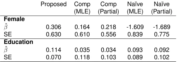
TABLE 3.3 : Data Example Log Hazard Ratio and Standard Error Estimates . . . 36

TABLE 4.1 : Power Estimated by Formula 4.3 and by Simulations fordV up to 100 . . . . 45

TABLE 4.2 : Power Estimated by Formula 4.3 and by Simulations fordV up to 200 . . . . 46

TABLE 4.3 : Optimal Number of Events in Study Design Example . . . 48

TABLE A.1 : Simulation Results for Type 1 Censoring andn= 500 . . . 62

TABLE A.2 : Simulation Results for Random Censoring andn= 500 . . . 63

LIST OF ILLUSTRATIONS

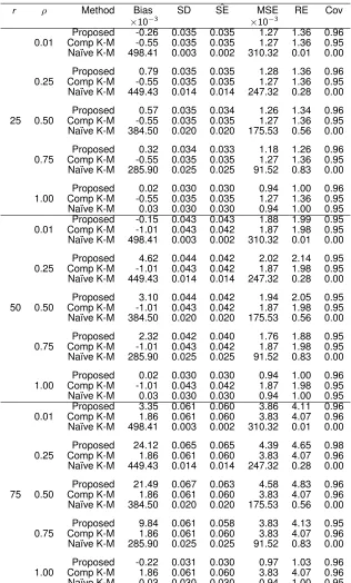
FIGURE 2.1 : Relative Efficiencies by Correlation Between True and Uncertain Endpoints (ρ) and Amount of Missingness of True Endpoints . . . 17 FIGURE 2.2 : Data Example Survival Function Estimates for Time to AD . . . 22

CHAPTER 1

I

In many clinical trials and epidemiological studies, the outcome of interest is time to an event, such

as disease progression. The true outcome in these studies is often too invasive or costly to

ob-tain, but alternative outcomes measure the true outcome with error. For example, the gold standard

method for assessing time to renal function halving measures glomerular filtration rate (GFR), which

is expensive and cumbersome to patients, but using equations based on serum creatinine to

esti-mate GFR is inexact (Stevens et al., 2006). Another example is in the time to pathological diagnosis

of Alzheimer’s disease (AD), which can be accurately obtained with a cerebral spinal fluid (CSF)

assay of amyloid beta (Aβ) protein concentrations (Shaw et al., 2009), but the lumbar puncture required for the procedure is often considered too painful for patients. An alternative method of AD

diagnosis more widely used in practice is based on evaluation of clinical symptoms and cognitive

tests, but the symptoms of AD are often mistaken for other types of dementia (Jack Jr et al., 2010).

Sometimes, it is possible to obtain both the uncertain or mismeasured outcome on all patients and

the true outcome on just a subset of patients. For these situations, it is important to develop powerful

analytical approaches to use the combined data, since standard methods for conducting survival

analysis utilize only one endpoint. This dissertation will develop innovative statistical methods to

conduct analyses on discrete time-to-event data with these characteristics. The proposed approach

can estimate survival functions and hazard ratios for the effects of binary or continuous covariates,

and it is shown to be superior to standard approaches that use only one of the outcomes. Optimal

study design strategies for designing new studies to implement the proposed method are also

developed.

1.1. Background

1.1.1. Methods with Uncertain Endpoints

When true outcomes are difficult to obtain, uncertain outcomes are often used as an alternative due

to their wide availability. Standard survival analysis methods, such as the Kaplan-Meier estimate of

biased results when using these uncertain outcomes. Several novel statistical methods have been

proposed to address this issue, but many rely on prior knowledge of the mismeasurement rates of

the uncertain endpoint.

Snapinn (1998) used weights representing certainty of potential endpoints to modify the Cox

pro-portional hazards model. Each of these weights are based on posterior probabilities that the

po-tential endpoint is a true endpoint, which rely either on assumptions about the characteristics of

the diagnostic tools or on an “endpoint committee” who must estimate them. As Snapinn

indi-cates, however, it may be difficult to obtain the appropriate weights accurately, which diminishes

the method’s performance (Snapinn, 1998).

Richardson and Hughes (2000) developed Expectation-Maximization (EM) algorithms for

estimat-ing the distribution of time to an event usestimat-ing uncertain outcomes. Meier, Richardson, and Hughes

(2003) extended this work to a semiparametric version assuming a proportional hazards model.

Both methods produce less biased survival estimates than standard survival analysis methods

and use supplemented EM algorithms to estimate variance-covariance matrices of parameter

es-timates. Similarly, Balasubramanian and Lagakos (2001) assumed a known time-dependent

sen-sitivity function to estimate the distribution of the time to perinatal HIV transmission. However, all

of these methods rely on known rates of sensitivity and specificity of the diagnostic tool used to

determine the uncertain outcome. These rates may not be available and estimates may not be

accurate. Magaret (2008) showed that even a 2 percent inaccuracy of specificity can cause a 14.5

percent bias in parameter estimates.

1.1.2. Use of a Validation Subsample

Although uncertain outcomes are mismeasured and can lead to biased parameter estimates, true

outcomes may also be available for a subset of patients. Using standard analysis methods on just

the true outcomes limits the sample size and therefore power in making inference. However,

statis-tical methods have been developed for the situation where both uncertain outcomes are available

on all patients and true outcomes available in a subset, known as a validation subsample.

Specifi-cally, Pepe (1992) developed an estimated likelihood method for these types of data, although not

specifically for a survival setting.

estimated likelihood takes the following form:

ˆ

L(β) =Y

i∈V

Pβ(Yi|Zi) Y

j∈V¯ Z

y

Pβ(y|Z) ˆP(S|y,Z)dy (1.1)

whereV represents the validation subsample, the set of patients who have both true and uncertain

outcomes, V¯ represents the non-validation set, in which patients only have uncertain outcomes,

andPˆ(S|y,Z)is estimated empirically (Pepe, 1992). Therefore, those who have the true outcomes

contribute the probability distribution of the true outcomes, as in a standard likelihood. Those who

only have the uncertain outcomes contribute an estimated probability distribution of the uncertain

outcomes, which incorporates the relationship between the true and uncertain outcomes. This

relationship is estimated by observing the values of the true and uncertain outcomes within the

validation subsample.

Although Pepe’s original work was not designed for survival outcomes, Fleming et al. (1994) used

the estimated likelihood method for the proportional hazards model by incorporating a validation set

available on all subjects (i.e., no missing true endpoint measures). In this special case, having the

uncertain outcomes is only useful in augmenting the likelihood for subjects with censored true failure

times. Magaret (2008) also extended Pepe’s work to the discrete proportional hazards model for

situations where outcomes are only validated when the uncertain event status is positive. Therefore,

Magaret’s method is useful for data with only a subsample of true outcomes, but it does not allow

for any false negatives. In addition, the method assumes there are no missed visits, so only type 1

right censoring (i.e., censoring time is not random) is allowed. Finally, the method only considers

discrete covariates of interest.

1.1.3. Study Design

Several methods exist to compute sample size for standard survival analysis studies (Freedman,

1982; Lakatos, 1986, 1988; Schoenfeld, 1981, 1983; Shih, 1995). Freedman (1982) developed

a sample size formula for the logrank test and compared the power calculated by the formula to

that using Monte Carlo simulations to show that the formula worked well. Schoenfeld (1981; 1983)

developed a similar formula for use with either a logrank test or a Cox proportional hazards model,

derived by exploiting asymptotic properties of the corresponding score test statistics. Both sample

methods are for single outcomes and do not take into account any potential mismeasurement.

1.2. Novel Developments

In this dissertation, we fill in the gaps in the literature by developing flexible methods for the design

and analysis of time-to-event data with uncertain outcomes using a validation subsample. The

dis-sertation consists of three parts. In Chapter 2, we first propose a nonparametric discrete survival

function estimator. There are three new contributions to the literature from this paper which we

summarize below. First, we propose a maximum estimated likelihood estimator that incorporates

both uncertain outcomes on all subjects and true outcomes on a validation subsample without

as-suming known mismeasurement rates of the uncertain outcomes. We assume study subjects are

evaluated at predetermined time points by study design, so survival time is a discrete random

vari-able for both true and uncertain endpoints. Second, we allow for missingness of the true outcome

regardless of the value of the uncertain event indicator, so both false negatives and false positives

are allowed. Third, our proposed estimator is able to handle both type 1 and random right

cen-soring mechanisms. We develop the asymptotic distribution theory for the proposed estimator and

provide an asymptotic variance estimator. We also demonstrate the performance of our proposed

estimator through extensive simulations and illustrate the use of the method by estimating the

sur-vival function for the time to AD diagnosis using data from the Alzheimer’s Disease Neuroimaging

Initiative (ADNI).

In Chapter 3, we develop a semiparametric approach to estimate a hazard ratio representing the

effect of a covariate of interest assuming a proportional hazards model. In addition to the

contri-butions to the literature above, the method discussed in this chapter allows for either a binary or a

continuous covariate. Unlike in previous literature and in the nonparametric version, the estimated

likelihood that incorporates a continuous covariate requires the use of a smooth kernel-type

func-tion in estimafunc-tion. For both the binary and continuous covariate cases, we develop the asymptotic

theory for the estimate of the log hazard ratio and its asymptotic variance estimator while treating all

other parameters as nuisance parameters. We test the semiparametric estimated likelihood method

using extensive simulations. Finally, using the ADNI data, we illustrate the method by estimating

the effect of gender (binary) and years of education (continuous) on time to AD diagnosis.

validation subsample when using the semiparametric estimated likelihood method to assess

treat-ment effects. We calculate sample sizes assuming the goal is to achieve a pre-specified power for a

Wald-type test to detect differences between treatment groups. We develop optimal designs based

on simulations for a range of study conditions, including varying effect sizes, correlations between

outcomes, percentage of missing true outcomes, number of time points in the study, and baseline

distributions. We also propose the use of a sample size formula adapted from Schoenfeld’s (1983)

formula for the Cox proportional hazards model and demonstrate its performance by comparing

calculated power to those from Monte Carlo simulations. Finally, we conclude in Chapter 5 and

CHAPTER 2

N

D

S

F

E

U

E

U

I

V

S

2.1. Introduction

Survival function estimation is crucial in studying disease progression and therapeutic benefits of

drugs in epidemiology studies and clinical trials that involve time-to-event data. However, event

outcomes may be subject to measurement error, which can lead to misclassification of the true

event outcome. Gold standard or better outcome measurements are sometimes unavailable due

to high costs or invasive procedures, and using only complete, true outcomes may exclude many

subjects due to missing data. For example, the pathological diagnosis of Alzheimer’s disease (AD)

has been traditionally determined by autopsy. Recently, as we enter the exciting new era of

“per-sonalized medicine,” AD biomarker research has been very successful. It is well accepted now that

time to pathological diagnosis of AD can be reliably measured by time to an abnormal biomarker

value among living participants in research studies (Shaw et al., 2009). Specifically, the amyloid

beta (Aβ) protein biomarker from a cerebral spinal fluid (CSF) assay has been shown to represent the pathological aspects of AD well and the abnormality of Aβ can be used as a reliable (true) endpoint for studying time to pathological diagnosis of AD among living participants (Shaw et al.,

2009). However, the CSF biomarker assay involves a lumbar puncture, so it is often considered

too invasive for many patients and therefore has limited availability. An alternative outcome is time

to diagnosis of AD by clinical assessment, which relies primarily on cognitive tests. The clinical

diagnosis is widely available, but it measures the outcome of pathological diagnosis with error.

Sources of error in clinical diagnosis include normal aging independent of AD, “cognitive reserve”

due to education-linked factors, and disease heterogeneity (Nelson et al., 2012). Thus, the clinical

diagnosis is an uncertain endpoint. Under these circumstances, it is important to develop powerful

analytical approaches to use combined information from both true and uncertain endpoints to

ob-tain consistent and more efficient estimators compared to the na¨ıve estimator, which ignores true

endpoint measures, and the complete-case estimator, which uses only the available true endpoint

Our proposed method is motivated by survival function estimation of time to pathological

develop-ment of AD using data from the Alzheimer’s Disease Neuroimaging Initiative (ADNI) (Weiner et al.,

2012). Participants in the ongoing ADNI study were evaluated at predetermined time points to

as-sess AD development based on cognitive tests. Regardless of these clinical diagnoses, a subset

of participants also had longitudinal CSF assays to measureAβ values, from which time to CSF diagnoses could be determined. Some study participants randomly withdrew from the study

be-fore developing cognitive or pathological signs of AD. Therebe-fore, survival time is a discrete random

variable subject to random right censoring. Although several nonparametric and semiparametric

methods for estimating survival outcomes when the outcome is uncertain have been proposed,

many rely on prior knowledge of the mismeasurement rates of the uncertain endpoint without an

in-ternal validation subsample of true endpoints (Snapinn, 1998; Richardson and Hughes, 2000; Meier

et al., 2003; Balasubramanian and Lagakos, 2001). Among those that do incorporate a validation

subsample, the method primarily focused on the discrete proportional hazards model requiring that

validation is only performed on those with positive uncertain endpoints, and the method cannot

handle the random censoring we have in the ADNI data (Magaret, 2008).

Specifically, Snapinn (1998) estimated weights representing certainty of potential endpoints to

mod-ify the Cox proportional hazards model. Richardson and Hughes (2000) obtained unbiased

prod-uct limit estimates of time to an event when the event indicator has measurement error using an

Expectation-Maximization (EM) algorithm. Their estimate uses known information about the

sensi-tivity and specificity of the diagnostic test for having the event without a validation sample. Meier,

Richardson, and Hughes (2003) extended this work for the adjusted proportional hazards model

for discrete failure times, also assuming known sensitivity and specificity. Similarly,

Balasubrama-nian and Lagakos (2001) assumed a known time-dependent sensitivity function to estimate the

distribution of the time to perinatal HIV transmission.

Pepe (1992) developed an estimated likelihood method to incorporate both uncertain endpoints

and a validation subsample to make inference without assuming known sensitivity or specificity, but

not specifically for a survival setting. Fleming et al. (1994) used Pepe’s method for the proportional

hazards model by incorporating a validation set available on all subjects (i.e., no missing true

end-point measures) to augment the likelihood for subjects with censored failure times. Magaret (2008)

situations where outcomes were only validated when the mismeasured event status was positive,

so false-negatives were not possible. Because the method assumes no missed visits, only type 1

right censoring (i.e., censoring time is not random) is allowed. Therefore, these previous methods

are unable to address the unique challenges seen in the ADNI data.

We propose a nonparametric discrete survival function estimator for data with characteristics

sim-ilar to those of the ADNI study. There are three new contributions to the literature from this paper

which we summarize below. First, we propose a nonparametric discrete survival function estimator

without assuming known mismeasurement rates of the uncertain outcome. Instead, we incorporate

information from an internal validation subsample to construct the survival function estimator. We

use Pepe’s (1992) framework to construct an estimated likelihood for the survival function of time

to an event, incorporating both an uncertain observed time and event indicator on all subjects and

a true observed time and event indicator on a validation subsample. The proposed estimator is

the nonparametric maximum estimated likelihood survival function estimator. In addition, because

study subjects are evaluated at predetermined time points by study design, survival time is a

dis-crete random variable for both true and uncertain endpoints. We develop the asymptotic distribution

theory and provide an asymptotic variance estimator. Second, the proposed nonparametric survival

function estimator allows missingness of the true endpoint regardless of the value of the uncertain

event indicator. In other words, validation can be conducted on subjects with either observed or

censored uncertain events. Third, the proposed estimator is able to handle both type 1 and random

right censoring mechanisms. Our allowance of random censoring and objective of estimating an

entire survival function provide some unique challenges in using survival outcomes as compared

to Pepe’s (1992) original work.

We organize the rest of the article as follows. We first describe the estimated likelihood and

non-parametric maximum estimated likelihood estimator (Section 2.2). We then develop the asymptotic

properties of the proposed estimator (Section 2.3). We perform extensive simulations to assess

the performance of our proposed estimator and compare it to the complete-case and na¨ıve

Kaplan-Meier survival function estimators (Section 2.4). The simulations consider different correlations

between true and uncertain endpoints, different amounts and types of censoring, as well as

differ-ent amounts of missingness of true endpoints. This is followed by an application to the estimation

ongoing ADNI study (Section 2.5). Finally, we summarize our findings and point to applications

where incorporating both true and uncertain endpoints are particularly useful (Section 2.6).

2.2. Proposed Nonparametric Maximum Estimated Likelihood Estimator

LetT represent the true time to event and C represent the true right censoring time, with event

indicator δ = I(T ≤ C). Similarly, let T∗ represent the uncertain time to event and C∗ be the uncertain right censoring time, with indicatorδ∗ =I(T∗ ≤C∗). DefineX = min{T,C}andX∗ = min{T∗,C∗}. ThenX andX∗represent the true and uncertain observed times, respectively. Letxk

represent thekth unique, ordered observed true time point fork = 1,· · ·,K, whereK is the total

number of unique true observed times. Let F represent the survival function of the true time to

event and letG represent the survival function of the true censoring time.

LetV represent the validation set, where both the uncertain and true outcomes are available. There

arenV subjects in the validation set. It is assumed that the validation subsample is a representative

sample of the entire cohort, implying that data are missing completely at random. ThenV¯ is the

non-validation set, where only the uncertain outcome is available and the true outcome is missing.

With a total ofnsubjects in the study, there aren−nV subjects in the non-validation set. The entire

observed data are(Xi,δi,Xi∗,δi∗)fori = 1,· · · ,nV and(Xj∗,δ∗j)forj = 1,· · ·,n−nV. Using similar arguments as in Pepe (1992), the full likelihood would then be

L=Y

i∈V

P(Xi,δi)P(Xi∗,δi∗|Xi,δi) Y

j∈V¯

P(X_j∗,δ∗_j). (2.1)

To avoid having to specify or assume the form of the relationship between the true and uncertain

endpoints, we propose to use the estimated likelihood

ˆ

L=Y

i∈V

P(Xi,δi) ˆP(Xi∗,δ

∗

i|Xi,δi) Y

j∈_V¯ ˆ

P(X_j∗,δ∗_j), (2.2)

where for discrete data,

ˆ

P(X_j∗,δ∗_j) =

K X

k=1 1 X

δ=0

P(xk,δ) ˆP(Xj∗,δ∗j|xk,δ). (2.3)

out-come, so the outer sum is taken over all possible time points,k = 1,· · ·,K. The estimated

condi-tional probabilityPˆ(X∗

j ,δ∗j|xk,δ)is given by

ˆ

P(X_j∗,δ∗_j|xk,δ) =

ˆ

P(X_j∗,δ_j∗,xk,δ)

ˆ

P(xk,δ)

(2.4)

= 1 nV

P i∈VI(X

∗

i =Xj∗,δi∗=δj∗,Xi =xk,δi=δ) 1

nV P

i∈VI(Xi=xk,δi =δ)

, (2.5)

whereI(·)is the indicator function. Conceptually, the conditional probability is estimated empirically

by counting the proportion of subjects in the validation set whose uncertain outcomes match those

of the given non-validation set subject. Because the conditional probabilityPˆ(X_i∗,δ_i∗|Xi,δi)from the validation set contribution does not contain any parameters, it can be factored out of the likelihood

and the estimated likelihood to be maximized becomes

ˆ

L∝Y

i∈V

P(Xi,δi) Y

j∈_V¯ ˆ

P(X_j∗,δ∗_j). (2.6)

Then for a subjecti ∈V, the contribution to the likelihood is the same as it would be in a standard

discrete survival setting,

P(Xi,δi) ={F(xki−1)−F(xki)}

δi_F(x

ki) 1−δi_G(x

ki−1)

δi_{G(x

ki−1)−G(xki)}

1−δi _(2.7)

∝ {F(xki−1)−F(xki)}

δi_F(x

ki)

1−δi _(2.8)

wherexki is the observed time for subjecti corresponding to thekth unique observed time point.

Only the true outcome contributes to the likelihood for those in the validation set, implying that

un-certain outcomes do not provide any additional information when the true outcome is known.

How-ever, the uncertain outcomes for those in the validation set are still used to estimate the relationship

between the uncertain and true outcomes, which are then used to weight likelihood contributions

for those in the non-validation set. For a subjectj∈V¯, the contribution to the likelihood is

ˆ

P(X_j∗,δ∗_j) =

K X k=1 1 X δ=0

{F(xk−1)−F(xk)}δF(xk)1−δG(xk−1)δ{G(xk−1)−G(xk)}1−δ·

1 nV

P

i∈V I(Xi∗=Xj∗,δi∗=δj∗,Xi=xk,δi =δ) 1

nV P

i∈VI(Xi =xk,δi=δ)

#

Unlike in the validation set contribution, the censoring distribution cannot be factored out of the

likelihood from the non-validation set contribution. This distribution is important in allowing random

censoring for survival outcomes in the estimated likelihood method. Note that any subjects in the

non-validation set with an observed uncertain time that does not match any observed uncertain

times in the validation set do not contribute to the likelihood.

There are two special cases worth considering. First, in the situation where the uncertain outcome

is perfect, orP(X,δ|X∗,δ∗) = 1, the likelihood reduces to that of the standard likelihood where all subjects have the true outcome. An example of this situation is when the uncertain outcome has

no measurement error or is exactly the same as the true outcome. Second, in the situation where

the uncertain outcome is useless, orP(X∗,δ∗|X,δ) = P(X∗,δ∗), the likelihood reduces to that of the standard likelihood where there is no non-validation set. Additional details on the derivation of

the estimated likelihood and on these special cases are available in Appendix A.1.

The estimated likelihood is a function of possible survival function values for the event distribution

and censoring distribution at each time point. The parameters representing the censoring

distribu-tionG are estimated jointly with the parameters representing the event distributionF, but treated

as nuisance parameters. When the study only has type 1 right censoring, though, the contribution

to the likelihood by the censoring distribution will always be 1, so the censoring distribution can be

factored out of the likelihood and does not need to be estimated. In order to solve for the

nonpara-metric maximum estimated likelihood survival function estimatorF using the estimated likelihood

we developed, we first note that the maximum estimate will be a step function that is continuous

from the right with left limits that falls only at event times observed in the validation set,t1,· · ·,t_K˜,

whereK˜ is the number of unique true event times. Similarly, if the censoring distribution is being

estimated, the maximum estimator will be a step function that is continuous from the right with left

limits that falls only at censoring times observed in the validation set. To solve for the parameters,

we used the Nelder-Mead algorithm to conduct constrained maximization. We required that both

F andG survival functions are monotonically non-increasing as time increases and are bounded

between 0 and 1. In the case where the parameter space is one-dimensional, meaning there is only

one observed event time in the validation set data and only type 1 censoring, we used the Brent

al-gorithm. To obtain initial estimates for the event distribution parameters, we used the complete-case

vali-dation set. Initial parameters for the censoring distribution were determined by the complete-case

Kaplan-Meier estimates calculated by inverting the event indicator to obtain a censoring indicator.

LetFˆ(t_k˜)represent the event distribution estimates obtained from the algorithm fork˜ = 1,· · ·, ˜K.

The maximum estimated likelihood survival function estimator is then the step function that takes

value 1 in the interval[0,t1),Fˆ(t˜_k)in each interval[t˜_k,t_k˜₊₁)fork˜ = 1,· · · , ˜K −1, andFˆ(t_K˜)in the

interval [t_K˜,xK], where xK is the last true observed time and may be equal tot_K˜ if a true event

occurs at the last true observed time. The estimator is considered undefined afterxK.

2.3. Asymptotic Properties of the Proposed Nonparametric Maximum Estimated

Likelihood Estimator

The asymptotic properties of the proposed estimator refer to the situation when the total number of

subjectsn→ ∞. As long as the proportion of subjects in the validation set to the total number of

subjects does not have a zero limit,limn→∞n_nv =pV >0, similar arguments as in Theorem 3.1 of Pepe (1992) imply thatFˆ(t)is a consistent estimator forF(t)for all timest. AlthoughFˆ(t)is only

estimated at observed event times,t1,· · ·,t_K˜, this set of observed event times will approach the set

of all possible observed event times, orK˜ →K asn→ ∞. Because we have discrete time points,

F(t)is also a step function that can be defined by the survival function values at each time point,

F(t1),· · · ,F(tK), and we have that

√ n                   ˆ

F(t1)

ˆ

F(t2) .. . ˆ

F(tK)          −         

F(t1)

F(t2) .. .

F(tK)                  

converges to a zero-mean Gaussian random variable in distribution with asymptotic variance

co-variance matrix equal toΣF, whereΣF is the top leftK×K quadrant of the full variance covariance

matrix

Σ =I−1₊(1−pV)2

pV

I−1_KI−1_,

whereIis the information matrix based on the (non-estimated) log likelihood andKis the expected

conditional variance of the non-validation contribution to the log likelihood (Pepe, 1992),

K=E

Var

_∂logP(X∗_,δ∗₎

∂θ

X,δ

(2.11)

for parameters θ = {F,G}. The first term in theΣ variance expression represents the variance component based on the maximum likelihood estimator and the second term represents a penalty

from estimating the likelihood with empirical probabilities. TheIandKmatrices can be estimated

consistently by

ˆ

I = 1

n

∂2_{log ˆL}

∂θ2 _{θ= ˆθ} (2.12)

for maximum estimated likelihood estimatesθˆ={Fˆ, ˆG}and

ˆ

K= 1

nV X

i∈V

ˆ

QiQˆiT θ= ˆθ , (2.13) where ˆ

Qi=

1

n−nV

1 ˆ

P(Xi,δi) X

j∈V¯ "

n

I(X_j∗=X_i∗,δ_j∗=δ∗_i)−_Pˆ_(X∗

j ,δ∗j|Xi,δi) o

·

(

D(Xi,δi)

ˆ

P(X∗

j ,δ∗j)

−

ˆ

D(X_j∗,δ_j∗) ˆ

P2_(X∗

j ,δj∗)

P(Xi,δi) )#

(2.14)

and

D(Xi,δi) =

∂P(Xi,δi)

∂θ (2.15)

ˆ

D(X_j∗,δ_j∗) =

K X k=1 1 X δ=0

∂P(X,δ)

∂θ

ˆ

P(X_j∗,δ∗_j|X,δ). (2.16)

In practice, derivatives in the variance expression can be calculated numerically. We found that

the numerical derivatives were sometimes unable to be computed or led to negative variances with

data that had large amounts of missingness or large numbers of parameters to estimate. In these

cases, bootstrapped variance estimates can be calculated or analytical forms of the derivatives

2.4. Simulations

Our proposed survival function estimator is motivated by the fact that true endpoints are missing

for some subjects while uncertain endpoints are available for all subjects and carry useful

informa-tion for survival funcinforma-tion estimainforma-tion. In order to assess the performance of our proposed survival

function estimator, we conducted a series of simulation studies. We simulated the true event time

from a discrete uniform distribution,T ∼Unif[1, 8], where survival time can only take integer values,

and assumed right censoring atC = 7. The uncertain time to event was calculated asT∗ =T +, where∼Unif[0,ζ]andis independent ofT. The maximum integer value of the discrete uniform distribution forwas calculated asζ=jq63·1−ρ2

ρ2 + 1−1

k

, wherebacrepresents the largest

inte-ger not greater thana, whereρrepresents the correlation betweenT andT∗. The expression for

ζ was computed using the definition of correlation betweenT andT∗, independence ofandT, and variance expressions forT and. Mathematical details of the derivation can be found in Ap-pendix A.2. We considered correlations ofρ∈ {0.01, 0.25, 0.50, 0.75, 1}. We set the right-censoring time for the uncertain endpoint also at C∗ = 7. To create a representative validation

subsam-ple, we simulated data missing completely at random (MCAR) by randomly selecting a proportion

r ∈ {0.25, 0.50, 0.75} of the sample to be missing true endpoints. We used total sample sizes of

n∈ {200, 500}and conducted 500 repetitions of the simulation for each set of parameter values.

For each simulation, we used the proposed method to calculate survival function estimates at

each observed time. We also calculated complete-case Kaplan-Meier estimates using only true

endpoints in the validation set, the na¨ıve Kaplan-Meier estimates using only uncertain endpoints

from all subjects, and the true Kaplan-Meier estimates using true endpoints from all subjects

(which would be unavailable in real data). For the proposed estimator, the complete-case

Kaplan-Meier estimator, and the na¨ıve Kaplan-Kaplan-Meier estimator, we calculated estimated bias (parameter

estimate−true parameter values), observed sample standard deviations (SD), estimated standard

errors (SE), relative efficiency (RE) compared to the true Kaplan-Meier estimator (where lower REˆ

implies greater efficiency and RE equal to 1 implies optimal efficiency), mean squared error (MSE)

estimates, and 95% coverage (Cov) at each of the observed time points. Each statistic was then

averaged over all time points. We note that for all simulations presented in Tables 2.1, 2.2, and 2.3,

the observed sample standard deviation corresponds well with the standard error estimates from

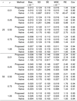
Table 2.1 shows the results from the simulation study with type 1 censoring and n = 200. The

proposed estimator behaves similarly to the complete-case Kaplan-Meier estimator in terms of

bias. Both have little bias, whereas the na¨ıve Kaplan-Meier estimator is heavily biased. When

the proportion of missingness is low or moderate (r = 0.25 or r = 0.50), the relative efficiency

of our proposed estimator is similar to that of the complete-case Kaplan-Meier estimator when

correlation is low and improves until it reaches optimal efficiency with correlation of 1, which can be

interpreted as the situation where the uncertain outcome has no measurement error. The MSE of

the proposed estimator is also similar to then becomes smaller than the MSE of the complete-case

Kaplan-Meier estimator as correlation increases, and it is consistently smaller than the MSE of the

na¨ıve Kaplan-Meier estimator. This demonstrates that using the internal validation subsample can

reduce the bias of survival estimates compared to using only uncertain endpoints and that using

uncertain endpoints in the non-validation subsample can improve efficiency compared to using

only true endpoints. When the amount of missing true outcomes is high (r = 0.75), though, our

proposed estimator is actually slightly less efficient than the complete-case Kaplan-Meier estimator

at low correlations between outcomes.

We saw similar results for simulations with n = 500, as shown in Appendix A.4. In addition, we

tested the performance of our method at smaller sample sizes,n∈ {10, 20, 30,· · · }, to determine

an approximate threshold for the number of subjects per parameter or events per variable (EPV)

needed for estimation. We calculated the EPV as the smallest number of events in the validation

set divided by 7, the number of parameters to estimate, such that average bias was less than 0.01

and average coverage was between 93% and 97%. Through these simulation studies, we found

an EPV of 4. We also increased the proportion of censored subjects (results not shown) by setting

an earlier censoring time for both endpoints and arrived at the same conclusions. Although we

assumed only non-negative measurement error of the uncertain endpoint for our simulations to

demonstrate the potentially large bias in the na¨ıve estimator and to better control the correlation

between outcomes, we also conducted simulations allowing for negative or positive measurement

error and the results (not shown) for our estimator and the complete-case estimator are similar.

To compare the efficiency between our proposed estimator and the complete-case Kaplan-Meier

estimator over various amounts of missingness, we computed the relative efficiencies (averaged

Table 2.1: Simulation Results for Type 1 Censoring andn= 200

r ρ Method Bias SD SEˆ MSE RE Cov

×10−3 _×10−3

0.01

Proposed -0.26 0.035 0.035 1.27 1.36 0.96 Comp K-M -0.55 0.035 0.035 1.27 1.36 0.95 Na¨ıve K-M 498.41 0.003 0.002 310.32 0.01 0.00

0.25

Proposed 0.79 0.035 0.035 1.28 1.36 0.96 Comp K-M -0.55 0.035 0.035 1.27 1.36 0.95 Na¨ıve K-M 449.43 0.014 0.014 247.32 0.28 0.00

25 0.50

Proposed 0.57 0.035 0.034 1.26 1.34 0.96 Comp K-M -0.55 0.035 0.035 1.27 1.36 0.95 Na¨ıve K-M 384.50 0.020 0.020 175.53 0.56 0.00

0.75

Proposed 0.32 0.034 0.033 1.18 1.26 0.96 Comp K-M -0.55 0.035 0.035 1.27 1.36 0.95 Na¨ıve K-M 285.90 0.025 0.025 91.52 0.83 0.00

1.00

Proposed 0.02 0.030 0.030 0.94 1.00 0.96 Comp K-M -0.55 0.035 0.035 1.27 1.36 0.95 Na¨ıve K-M 0.03 0.030 0.030 0.94 1.00 0.95

0.01

Proposed -0.15 0.043 0.043 1.88 1.99 0.95 Comp K-M -1.01 0.043 0.042 1.87 1.98 0.95 Na¨ıve K-M 498.41 0.003 0.002 310.32 0.01 0.00

0.25

Proposed 4.62 0.044 0.042 2.02 2.14 0.95 Comp K-M -1.01 0.043 0.042 1.87 1.98 0.95 Na¨ıve K-M 449.43 0.014 0.014 247.32 0.28 0.00

50 0.50

Proposed 3.10 0.044 0.042 1.94 2.05 0.95 Comp K-M -1.01 0.043 0.042 1.87 1.98 0.95 Na¨ıve K-M 384.50 0.020 0.020 175.53 0.56 0.00

0.75

Proposed 2.32 0.042 0.040 1.76 1.88 0.95 Comp K-M -1.01 0.043 0.042 1.87 1.98 0.95 Na¨ıve K-M 285.90 0.025 0.025 91.52 0.83 0.00

1.00

Proposed 0.02 0.030 0.030 0.94 1.00 0.96 Comp K-M -1.01 0.043 0.042 1.87 1.98 0.95 Na¨ıve K-M 0.03 0.030 0.030 0.94 1.00 0.95

0.01

Proposed 3.35 0.061 0.060 3.86 4.11 0.96 Comp K-M 1.86 0.061 0.060 3.83 4.07 0.96 Na¨ıve K-M 498.41 0.003 0.002 310.32 0.01 0.00

0.25

Proposed 24.12 0.065 0.065 4.39 4.65 0.98 Comp K-M 1.86 0.061 0.060 3.83 4.07 0.96 Na¨ıve K-M 449.43 0.014 0.014 247.32 0.28 0.00

75 0.50

Proposed 21.49 0.067 0.063 4.58 4.83 0.96 Comp K-M 1.86 0.061 0.060 3.83 4.07 0.96 Na¨ıve K-M 384.50 0.020 0.020 175.53 0.56 0.00

0.75

Proposed 9.84 0.061 0.058 3.83 4.13 0.95 Comp K-M 1.86 0.061 0.060 3.83 4.07 0.96 Na¨ıve K-M 285.90 0.025 0.025 91.52 0.83 0.00

1.00

Proposed -0.22 0.031 0.030 0.97 1.03 0.96 Comp K-M 1.86 0.061 0.060 3.83 4.07 0.96 Na¨ıve K-M 0.03 0.030 0.030 0.94 1.00 0.95

ρ∈ {0.25, 0.50, 0.75}(Figure 2.1). For these simulations, we used a larger sample size ofn= 500to ensure that the EPV was adequate even at the largest amounts of missingness. For correlations of

0.50 and 0.75, our proposed estimator is more efficient (lower RE) than the complete-case

Kaplan-Meier estimator when the proportion of missing data is low, then the efficiency curves cross and

our proposed estimator becomes less efficient. The point of crossing is at a higher percentage of

missingness with higher values of the correlation between outcomes. Even with low correlation (ρ= 0.25) between outcomes, though, our estimator has similar or lower efficiency than the

complete-case Kaplan-Meier estimator when the amount of missingness is 50% or less. This is consistent

with Pepe’s recommendation for non-survival data with one parameter of interest (Pepe, 1992).

Figure 2.1: Relative Efficiencies by Correlation Between True and Uncertain Endpoints (ρ) and Amount of Missingness of True Endpoints

0

20

40

60

80

ρ

=0.25

% Missing

1

2

3

4

5

6

7

0

20

40

60

80

ρ

=0.50

% Missing

1

2

3

4

5

6

7

0

20

40

60

80

ρ

=0.75

% Missing

1

2

3

4

5

6

7

Proposed

Comp K−M

A

v

er

age Relativ

e Efficiency

Proposed refers to the proposed estimator and Comp K-M refers to the complete-case Kaplan-Meier estimator. This figure appears in color in the electronic version of this article.

We explored the behavior of our proposed estimator under random censorship by simulating true

censor-ing times C ∼Unif[5, 7], and uncertain censoring times C∗ = C +γ whereγ ∼Unif[0, 2]. These simulations resulted in a small amount of censoring (approximately 30%). We also increased the

amount of censoring by simulating true censoring timesC ∼Unif[3, 7], which resulted in a larger

amount of censoring (approximately 50%). The results of these random censoring simulations are

shown in Table 2.2. Similar to the results from type 1 censoring, our proposed estimator has little

bias compared to the na¨ıve Kaplan-Meier estimator and is more efficient than the complete-case

Kaplan-Meier estimator for both small and large amounts of censoring. We saw similar results with

n= 500as seen in Appendix A.5.

Table 2.2: Simulation Results for Random Censoring andn= 200

r C Method Bias SD SEˆ MSE RE Cov

×10−3 _×10−3

25 S

Proposed 0.24 0.035 0.034 1.25 1.17 0.96 Comp K-M 0.39 0.038 0.037 1.47 1.39 0.95 Na¨ıve K-M 119.63 0.030 0.029 15.47 0.83 0.03

L

Proposed 0.57 0.040 0.038 1.65 1.20 0.96 Comp K-M 0.37 0.043 0.041 1.94 1.44 0.94 Na¨ıve K-M 119.98 0.032 0.032 15.75 0.78 0.05

50 S

Proposed -2.18 0.040 0.041 1.64 1.54 0.95 Comp K-M -0.12 0.047 0.046 2.23 2.10 0.95 Na¨ıve K-M 119.63 0.03 0.029 15.47 0.83 0.03

L

Proposed -1.99 0.049 0.044 2.68 1.84 0.96 Comp K-M -0.52 0.053 0.050 2.95 2.18 0.93 Na¨ıve K-M 119.98 0.032 0.032 15.75 0.78 0.05

ris the percent missing andCis the amount of censoring, where S means small (30%) and L means large (50%). Proposed refers to the proposed estimator, Comp K-M refers to the complete-case Kaplan-Meier estimator, and Na¨ıve K-M refers to the na¨ıve Kaplan-Meier estimator. SD is standard deviation of estimates across simulations,SE is estimated standard error of the estimate, MSE is mean squared error, RE is relativeˆ efficiency, Cov is 95% coverage, all averaged across time.

To test the robustness of the MCAR assumption of the proposed method, we relaxed this

assump-tion and simulated data missing at random (MAR). We defined a missingness indicatorR, where

the uncertain indicatorδ∗such that

R|(δ∗= 0) =

  

 

1 with probabilitypR

0 with probability1−pR

R|(δ∗= 1) =

  

 

1 with probability1−pR

0 with probabilitypR

for probability pR = 0.60. This implies that the probability of missingness of the true endpoint

depends on the observed censoring indicator of the uncertain endpoint. In the AD example, this

would imply that subjects who are clinically determined to be non-AD during the study are more

likely to miss the CSF biomarker endpoint. In the results from the MAR data in Table 2.3, we

see that both the proposed estimator and the complete-case Kaplan-Meier estimator is sometimes

slightly biased. However, the proposed estimator is less biased than the complete-case

Kaplan-Meier estimator, particularly when the correlation between outcomes is very high. Because of

these differences in bias, the coverage of the proposed estimator is better than the coverage of

the complete-case Kaplan-Meier estimator when the correlation between outcomes is greater than

0.01. We saw similar results withn= 500as seen in Appendix A.6.

2.5. Application to the Alzheimer’s Disease Neuroimaging Initiative Study

We illustrated our method by considering data (retrieved on July 26, 2013) from the ongoing ADNI

study (Weiner et al., 2012). See Appendix A.3 for more detailed information about the ADNI study.

Participants in this study were seen every 6 months until the end of two years, then annually

there-after, at which time clinical diagnoses of non-AD (cognitively normal or MCI) or AD were assessed.

These follow-up times were predetermined by study design, and thus discrete survival estimates

would be appropriate in this study. The current study includes data from participants in the

ADNI-1 and ADNI-GO segments of the ADNI study. For those who agreed to a lumbar puncture, CSF

assays were performed and Aβ protein concentrations were measured. Participants with anAβ

biomarker value greater than 192 pg/ml were classified as non-AD at baseline and those with an

Aβ value less than or equal to 192 pg/ml were classified as AD at baseline (Shaw et al., 2009). There were 186 patients who were non-AD at the time of enrollment according to both the

Table 2.3: Simulation Results for Data Missing at Random andn= 200

Censoring ρ/C Method Bias SD SEˆ MSE RE Cov

×10−3 _×10−3

0.01

Proposed 2.53 0.048 0.048 2.31 2.47 0.96 Comp K-M 0.91 0.048 0.048 2.31 2.47 0.95 Na¨ıve K-M 498.41 0.003 0.002 310.32 0.01 0.00

0.25

Proposed 17.06 0.048 0.049 2.38 2.56 0.97 Comp K-M -11.75 0.046 0.046 2.17 2.31 0.94 Na¨ıve K-M 449.43 0.014 0.014 247.32 0.28 0.00

Type 1 0.50

Proposed 21.47 0.047 0.046 2.22 2.38 0.98 Comp K-M -26.55 0.045 0.045 2.06 2.19 0.90 Na¨ıve K-M 384.50 0.020 0.020 175.53 0.56 0.00

0.75

Proposed 16.27 0.042 0.041 1.78 1.94 0.96 Comp K-M -44.30 0.043 0.042 1.89 2.00 0.81 Na¨ıve K-M 285.90 0.025 0.025 91.52 0.83 0.00

1.00

Proposed 0.02 0.030 0.030 0.94 1.00 0.96 Comp K-M -22.56 0.039 0.039 1.57 1.65 0.88 Na¨ıve K-M 0.03 0.030 0.030 0.94 1.00 0.95

Random S

Proposed 0.32 0.039 0.044 1.62 1.49 0.96 Comp K-M -33.92 0.043 0.042 1.87 1.78 0.86 Na¨ıve K-M 119.63 0.03 0.029 15.47 0.83 0.03

L

Proposed 1.66 0.047 0.044 2.49 1.69 0.96 Comp K-M -41.74 0.048 0.047 2.31 1.81 0.83 Na¨ıve K-M 119.98 0.032 0.032 15.75 0.78 0.05

Censoring is the type of the censoring mechanism andρ/C either represents the correlationρbetween true and uncertain outcomes or represents the amount of censoring, where S means small (30%) and L means large (50%). Proposed refers to the proposed estimator, Comp K-M refers to the complete-case

recorded to obtain an uncertain, mismeasured outcome on all patients. A subset of 110 patients

continued to have CSF assays performed annually. For these 110 patients in the validation set,

patients were classified as non-AD or AD at each time point using the same cutoff of 192 pg/ml and

the true time to AD or last follow-up was also recorded. Thus, patients with any CSF assays during

up were considered to be in the validation set and those with no CSF assays during

follow-up were considered to be in the non-validation set, ornV = 110andn= 186using the notation of

Section 2.2.

First, we assessed the missingness mechanism in the data. We used a log-rank test to compare the

survival functions for time to clinical AD diagnosis between the non-validation set and the validation

set. Theχ2test statistic was 0.2 with 1 degree of freedom, yielding a p-value of 0.662. We also used Fisher’s exact test to test for an association between the clinical event indicator and missingness.

The p-value was 1. Further, because we used all available longitudinal CSF assays, those who

were missing CSF diagnoses were missing immediately after baseline. Since all subjects begin as

non-AD at baseline, the missingness could not be dependent on baseline CSF or clinical diagnoses.

Therefore, we did not find strong evidence against the MCAR assumption.

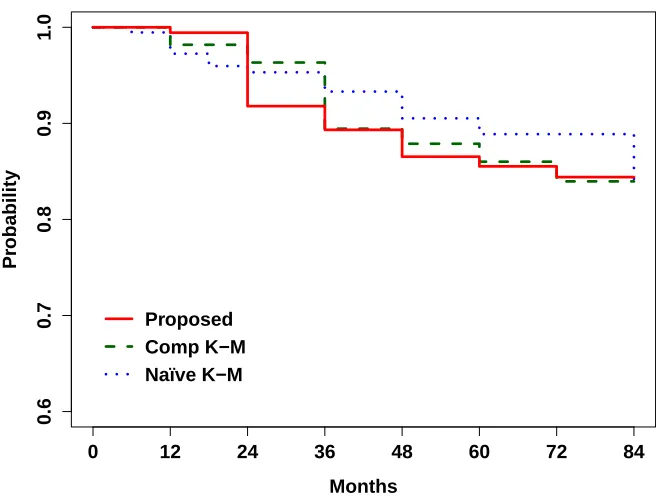
Figure 2.2 shows the estimated survival functions using our proposed estimator which maximized

the estimated likelihood, the complete-case Kaplan-Meier estimator which only uses 110 CSF

diag-noses, and the na¨ıve Kaplan-Meier estimator which only uses the 186 clinical diagnoses. The three

survival functions are very similar until 36 months, at which time the na¨ıve Kaplan-Meier estimate

begins to diverge from the other two survival curves. With higher survival probabilities, the na¨ıve

estimate overestimates the probability of being AD-free after 36 months compared to the proposed

estimator and complete-case Kaplan-Meier estimator. Since the na¨ıve estimate is based on only

clinical diagnoses, this would indicate that abnormality ofAβoccurred earlier than cognitive impair-ment. This finding is consistent with the recent theoretical model of AD pathology developed by

Jack et al. (2010).

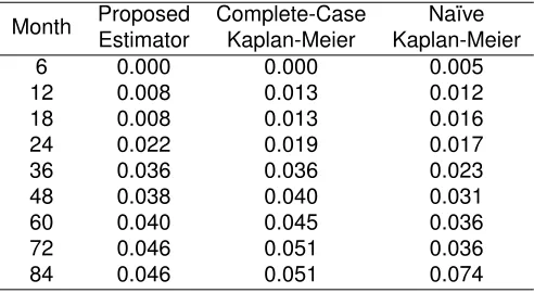
Table 2.4 shows the standard error estimates at each time point. The standard errors of the

pro-posed estimate are similar to or smaller than those of the complete-case Kaplan-Meier estimate at

all time points. This further supports the conclusion that the proposed estimator helps to improve

Figure 2.2: Data Example Survival Function Estimates for Time to AD

0.6

0.7

0.8

0.9

1.0

Months

Pr

obability

0 12 24 36 48 60 72 84

Proposed Comp K−M Naïve K−M

Proposed refers to the proposed estimator, Comp K-M refers to the complete-case Kaplan-Meier estimator, and Na¨ıve K-M refers to the na¨ıve Kaplan-Meier estimator. This figure appears in color in the electronic version of this article.

2.6. Discussion

We proposed a nonparametric maximum likelihood estimator for the discrete survival function in the

presence of uncertain endpoints by using an internal validation subsample. We allowed for random

censoring for survival outcomes by incorporating a censoring distribution in the likelihood, showed

that the survival function estimator is a step function that drops only at observed event times, and

proved that the proposed estimator is consistent and asymptotically normal at each discrete time

point. We evaluated the finite sample performance of the proposed estimator through extensive

simulations. We found that the proposed estimator has little bias and can improve efficiency

rela-tive to the complete-case Kaplan-Meier estimator. It can also reduce bias compared to the na¨ıve

Kaplan-Meier estimator. The proposed estimator also works better than the complete-case and

na¨ıve estimators under departure from the MCAR assumption.

Table 2.4: Data Example Standard Error Estimates

Month Proposed Complete-Case Na¨ıve Estimator Kaplan-Meier Kaplan-Meier 6 0.000 0.000 0.005 12 0.008 0.013 0.012 18 0.008 0.013 0.016 24 0.022 0.019 0.017 36 0.036 0.036 0.023 48 0.038 0.040 0.031 60 0.040 0.045 0.036 72 0.046 0.051 0.036 84 0.046 0.051 0.074

outcome may be costly to obtain on all subjects, but using the proposed method can incorporate

a less costly uncertain outcome assessed on all subjects and the true outcomes on a smaller

subsample. Compared to obtaining true outcomes on all subjects which can be very costly or using

a complete-case estimator on the smaller subsample, our estimator can reduce costs of the trial

without sacrificing power.

The proposed approach does not require that only subjects with positive uncertain endpoints (e.g.,

having clinical AD in our data example) can be validated in contrast to previous literature. Our

ap-proach allows that all subjects can have the opportunity to be validated. Through simulations, we

found that the efficiency gains of our proposed estimator depends on both the correlation between

the uncertain and true outcome and the size of the validation sample. However, in general, the

proposed estimator seems to work well when the size of the validation sample is 50% or more of

the total sample size. The proposed method can be used with data that have both type 1 right

censoring and random right censoring, whereas previous methods only allowed type 1 right

cen-soring. The proposed method also assumes that study subjects are seen at predetermined time

points and relies on a discrete time framework. In studies where subjects are evaluated at any time,

the proposed estimator may not improve efficiency compared to the complete-case Kaplan-Meier

estimator. For this situation, a modified approach must be developed.

The proposed method only estimates a single survival function. A natural extension of the method

would be a semiparametric version that is able to incorporate covariates and conduct

between-group comparisons. The extension of our proposed method for a proportional hazards model with

As early detection of Alzheimer’s disease and other chronic diseases becomes increasingly

impor-tant, but event outcomes may be hard to obtain for everyone, we recommend collecting an internal

validation sample when the measures of the event outcome are uncertain so that statistical analysis

CHAPTER 3

S

S

A

U

E

U

I

V

S

3.1. Introduction

In epidemiological studies and clinical trials, interest often lies in comparing the effects of

treat-ment on time to an event. The Cox proportional hazards model is a common, standard method of

survival analysis for analyzing true outcome data, but true outcomes are often unavailable due to

invasiveness or cost restrictions. For example, in the pathological diagnosis of Alzheimer’s disease

(AD), the outcome of interest may be a cerebral spinal fluid (CSF) diagnosis. However, the CSF

assay requires a lumbar puncture to measure Aβprotein concentrations in the spinal fluid, which is considered too painful for some patients. In these cases, true outcomes data may be supplemented

by alternative outcomes that measure the true outcomes with some error. In the case of

diagnos-ing AD, a clinical diagnosis based on cognitive tests may be used. The clinical diagnosis presents

differently from the CSF diagnosis and therefore measures the true outcome with error because

clinical symptoms of AD are easily mistaken for other types of dementia. However, clinical

diag-noses are more widely available than the CSF diagdiag-noses. Using both the uncertain, mismeasured

outcome on all subjects and the true outcome on a subsample of subjects, called the validation

sample, estimates of covariate effects can be improved.

Previous methods for estimating survival outcomes in these situations assumed known

mismea-surement rates of the uncertain outcome, allowed only positive uncertain outcomes to be validated

with an assessment of the true outcome, and/or only allowed for fixed censoring (Richardson and

Hughes, 2000; Meier et al., 2003; Balasubramanian and Lagakos, 2001; Magaret, 2008). For

ex-ample, Magaret (2008) adapted a method first introduced by Pepe (1992) for discrete survival data

and only discrete covariates using the proportional hazards model. Pepe’s method involved an

estimated likelihood method that incorporates information from both uncertain outcomes and true

outcomes, where estimation is performed for the conditional probability of the uncertain outcome

given the true outcome (Pepe, 1992). Zee and Xie (Chapter 2) adapted the estimated likelihood

fixed or random censoring mechanisms.

In this paper, we extend the work of Zee and Xie (Chapter 2, under revision for Biometrics) to a semiparametric estimated likelihood method to estimate a parameter representing a covariate

ef-fect for data with uncertain outcomes on all subjects and true outcomes on a subset. We assume

a proportional hazards model and estimate the log hazard ratio of the survival outcome comparing

different covariate values. Unlike Magaret’s (2008) method which only considered discrete

covari-ates of interest, we consider both a binary or a continuous covariate. Although we express our

approach with a binary categorical variable for ease of notation, the method can be easily modified

to consider categorical variables with more than two levels. For the continuous covariate, we use a

smooth kernel type estimator within the likelihood. The proposed estimator of the log hazard ratio

is consistent and asymptotically normal. The rest of the article is organized as follows. Section 3.2

describes the estimated likelihood and asymptotic properties for a binary covariate. Section 3.3

describes the method and asymptotic properties for a continuous covariate. Section 3.4 contains

results of our simulation study. In Section 3.5, we demonstrate the use of our method using data

from the Alzheimer’s Disease Neuroimaging Initiative to estimate covariate effects. Finally, we

sum-marize our results and discuss implications of using our proposed method in Section 3.6.

3.2. Semiparametric Estimated Likelihood with a Binary Covariate

3.2.1. Maximum Estimated Likelihood Estimation

LetT represent the true time to event and C represent the true right censoring time, with event

indicator δ = I(T ≤ C). Similarly, let T∗ represent the uncertain time to event and C∗ be the uncertain right censoring time, with indicatorδ∗ =I(T∗ ≤C∗). DefineX = min{T,C}andX∗ = min{T∗,C∗}. ThenX andX∗represent the true and uncertain observed times, respectively. LetXk

represent thekth unique, ordered observed true time point fork = 1,· · ·,K, whereK is the total

number of unique true observed times. LetF0represent the baseline survival function of the true

time to event. We assume a proportional hazards model withF(t) =F0(t)exp(βZ)whereZ ∈ {0, 1}is

the binary covariate of interest andβrepresents the log hazard ratio of the event comparingZ = 1 toZ = 0. We assume that the covariate is available for all subjects. Finally, we assume independent