On Clustering Algorithms: Applications in
Word-Embedding Documents
Israel Mendonça
1*, Antoine Trouvé
2, Akira Fukuda
1, Kazuaki Murakami
2 1 Kyushu University, 744-Motooka, Nishi-Ku, Fukuoka, Fukuoka, Japan.2 Team Aibod, 1-8-7-Daimyo, Chuo-Ku, Fukuoka, Fukuoka, Japan.
* Corresponding author. Tel.: +81-092-982-6090; email: [email protected]
Abstract: In this paper, we study the effectiveness of classical literature clustering algorithms applied to free text documents. We analyze the effects of varying the parameters on their performance and which aspects directly influence in the results. We apply a word-embedding-based technique to represent the document's bag-of-words and therefore be able to compare and study how these algorithms performs in the task of clustering these documents. We use two metrics that captures different aspects of the partitions and analyze those algorithms on the light of it. One of the main findings of this work is that some clustering algorithms are able to have a partition that's up to 91% of the real partition, whilst other performs really poor for the same dataset. We also find limitations on these techniques when trying to cluster hard datasets.
Key words: Clustering, natural-language-processing, word-embedding.
1.
Introduction
Document clustering is a fundamental tool for efficient organization, navigation, and retrieval of items in systems with a large amount of documents. A clustering technique quality is measured by their capacity of automatically separate items in a meaningful way, in the sense that items from the same group have similar properties and features, while items from different groups have strong dissimilar properties and features.
When clustering text documents, we need to select the appropriate form to represent documents, and the two most common ways to represent them are via bag of words (BOW), in which a document is represented as the set of its words; and term-frequency inverse document frequency (tf-idf), in which the importance of words in the document is measured against the importance of it on the corpora. However, as most of the clustering techniques rely on the notion of distance to separate the items, using any of those techniques becomes unfeasible.
Word2Vec models were first presented in 2013 by Mikolov et al. [1] and the main objective of their work was to generate word embedding that carries the semantic meaning of words. Word2Vec represent words as high-dimensional vectors. Different authors used word2vec to represent text documents due to the fact that they can be represented as a matrix or a single vector.
In this work, we use an approach similar to bag-of-words, by using all the words of the documents to represent it. We start by convert the document’s bag-of-words into the Word2Vec embedded version, which results in each document being represented as a matrix containing one word per row, and each row contains a word2vec feature, in a total of 300 columns (for Google’s one). A document is represented as a single vector with each column being the average of the corresponding column in the matrix.
Our main contribution is the analysis of the effectiveness of different clustering algorithms when applied into free text documents. We selected two real word datasets and then performed an empirical evaluation with them. Both datasets have different characteristics, which allowed us to compare different aspects of the algorithms. We use Normalized Mutual Information and Homogeneity scores to evaluate the overall quality of clustering solutions, which are commonly used metrics in clustering.
2.
Clustering
The problem of clustering consists in finding a partition of the elements of a set, such that individuals with higher similarity lies inside the same parts (clusters) and few lie in-between them. To measure the effectiveness of those techniques, we selected five algorithms for our experiments, which we briefly present here. All of them are able to process word-embedding document representation.
K-Means.[2] tries to cluster the points by first assigning random clusters to the points, and then perform several iterative update steps. Each step consists of computing the initial mean to be the centroid of the cluster's randomly assigned points. The update step is run until the group's centers doesn't change much from each iteration. Although this method converges fast O(n), it has two main setbacks: First is that the result is very dependent of the initialization step, which means that you need to run the same algorithm several times to have a good result. Second is that you need to specify the number of clusters beforehand, something that is not always desirable.
Expectation–Maximization (EM) Clustering using Gaussian Mixture Models (GMM). [3] assumes that the data points are Gaussian distributed, so that it describes the shape of clusters based on two parameters: The mean and the standard deviation. Since we have standard deviation both x and y axis, it means that clusters can take an elliptical shape. It starts by selecting random center points for each cluster. The second step is then compute the probability of each data point belong to each cluster. On the third step, it computes a new set of parameters for the Gaussian distributions such that we maximize the probabilities of data points within the clusters. The second and the third step are repeated until convergence. The main two advantages of GMM is that clusters can have an elliptical shape and also points can have more than one cluster (since the membership is a probability). The drawbacks are the same as for K-Means, like it depends of the initialization and you need to define a number of clusters beforehand.
Spectral Clustering.[4] creates a graph with the points in which each point is a vertex and the similarity of the points are weighted edges. It then computes the Laplacian of the adjacency matrix and then calculates the spectrum of the matrix, i.e. it's eigenvectors sorted from the most important one to the least important one. The idea of spectral clustering is to cluster the points using these keigenvectors as features. So, you take thekleast significative eigenvectors and you have your points in kdimensions. You then run a clustering algorithm like K-means to have your partition. The main advantage of this technique is that it is able to cluster points when K-means works badly because the clusters are not linearly separable in their original space. The main drawback is that it is dependent of other clustering techniques.
Mean Shift. [5] is a sliding-window-based algorithm that attempts to find dense areas of data points. Initially it will random several points on the search space, and each point will have a window of radius r
around it. The update step consists of moving the points to a region with more dense points within each point window. The algorithm converges when all the points are in the densest point within its window. The final step is to remove the overlapping windows preserving the one with more points. The data points are then clustered according to the sliding window in which they reside. The method converges fast and you don't have to specify the number of clusters but choosing the radius of the window can be non-trivial.
and then selects one of them at random. It then marks this point as noise or a cluster-point-candidate based on a pre-defined minimal number of epsilon distant-neighbors. The update step continues to find neighbors until there isn't cluster-point-candidates at epsilon distances. The process then restarts again in a non-visited
point until all points were visited. BDSCAN find noises and doesn't requires a pre-set number of clusters, but it doesn't scale well when the clusters vary in density.
3.
Experiments
3.1.
Dataset and Experimental Setup
We use two real world datasets with different characteristics to test the algorithms: BBC-Sports articles from 2004 to 2005, and Ohsumed: a collection of medical abstracts labeled by the kind of cardiovascular disease group. Table 1 presents relevant statistics for each of these training datasets including the number of files, number of classes and the number of words. For our experiments, we have chosen two sizes of clusters for the clustering algorithms: 5 and 10 clusters. For example, for the k-Means clustering, we used
k=5 and k=10. This doesn’t affect Mean Shift or DBSCAN because they do not require a pre-defined number of clusters. On DBSCAN we used epsilon as 0.75.
To compare the algorithms against the datasets, we selected two measures: Normalized Mutual Information (NMI), which is the standard measure to compare clustering techniques in the domain of unsupervised learning [7]. The outcomes of NMI range from -1 to 1, in which -1 represents completely different partitions, and 1 represents completely identical partitions, and 0 represents statistical independency. The higher the NMI score, the closer to the real label the partition is. The second measure is
Homogeneity, which can produce outcomes from -1 to 1 and measures how homogeneous is each cluster in the partition. The higher the homogeneity score, the better separated each cluster is.
We run our experiments using the Scikit-learn package for python and google's word2vec package to convert the words to embeddings.
Table 1. Datasets Details
Name Classes #Documents words
BBC-Sports 5 367 10676
Ohsumed 10 3999 30455
3.2.
BBC Sports
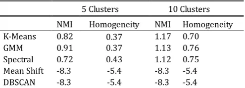
Table 2. BBC-Sports Dataset
5 Clusters 10 Clusters
NMI Homogeneity NMI Homogeneity
K-Means 0.82 0.37 1.17 0.70
GMM 0.91 0.37 1.13 0.76
Spectral 0.72 0.43 1.12 0.75
Mean Shift -8.3 -5.4 -8.3 -5.4
DBSCAN -8.3 -5.4 -8.3 -5.4
cluster. The existence of outliers is natural, since some information was lost during the conversion from the bag-of-words to the word-embedded version. One of the main reasons that the algorithms have a general score on this is due to the fact that the documents can be easily separated, since news about sports will usually have into its contents key-words that made them easily separable.
When we increase the number of clusters to 10, the NMI score goes beyond 1, this is because we have more clusters than the original labeling. The homogeneity increases by nearly 100% in the previous good algorithms, which can be explained by the fact that with more clusters, the tendency is that each cluster has less members, which makes the probability of a cluster having a foreign member, smaller.
Mean Shift and DBSCAN did not partition well the documents, even when we variated their input parameters, they instead placed all the documents inside a single cluster. This may be caused by the high dimensionality of the data. Each document in our approach was represented as a document of 300 dimensions. The results for both algorithms were poor in this dataset.
3.3.
Ohsumed
Table 3. Ohsumed
5 Clusters 10 Clusters
NMI Homogeneity NMI Homogeneity
K-Means 0.15 0.074 0.24 0.11
GMM 0.15 0.073 0.24 0.12
Spectral 0.09 0.05 0.08 0.04
Mean Shift -3.2 -1.6 -3.2 -1.6
DBSCAN -3.2 -4.4 -3.2 -4.4
The results for Ohsumed can be verified at Table 3. Differently from BBC-Sports, in this dataset, all the algorithms performed poorly for both settings (5 and 10 clusters), with the best of them scoring only 24% of the actual partition in the best case. Since Ohsumed has 10 classes, having a perfect score with only 5 clusters is an impossible task. When we add 5 more classes, the results increased in more than 50% for NMI, but the overall score is still far from the original partition. One of the reasons that may be curbing the performance of the algorithms, it is that Ohsumed contains a large number of technical medical words, which difficult the task of giving these words a context using the word-embedder. This may be affecting the way documents in Ohsumed are represented, and in the end hurting the performance of the clustering algorithms. Again, Mean Shift and DBSCAN were not able to separate the documents well and placed all the documents into a single cluster, which made their result worse than the K-Means, GMM and Spectral Clustering.
We performed a further analysis varying the parameters of our algorithm to try to get good results from Ohsumed. As similar to BBC-Sports, we verified how the algorithms would perform if we have the number of clusters double the number of pre-defined classes in the dataset. As for the NMI score, the increment was not so significant, but K-Means was able to go up to 32%, with GMM and Spectral Clustering having 30% and 16% respectively. The Homogeneity score increment was of 3%, which did not make much difference in the final score. On light of these facts, we can then conclude that these algorithms failed in separate well the documents, so there may have some other tuning or algorithms more suited for this dataset.
4.
Conclusion
BBC-Sports three out of the five algorithms had satisfactory results, with K-Means having 91% NMI score by having the same amount of clusters as pre-defined classes and 100% for double the number of classes. We then analyzed the performances of these algorithms for a difficult dataset, and none of them performed well, with again K-Means having the best performance among them. For both datasets, Mean-Shift and DBSCAN failed to separate the documents and placed all of them in a single cluster, which made their results being the worst.
We can conclude that the parameters of the algorithms greatly influences the results, in the sense that knowing the particularities of the datasets, or at least the number of classes it can be divided can give us good results. Some algorithms cannot be used together with word-embedded document representations because their performance is hurt by the high dimensionality of the representations.
Acknowledgment
The authors are grateful to the National Council of Scientific and Technologic Development (CNPQ) for its financial support through the Science Without Borders program, see (http://www.cienciasemfronteiras.gov.br).
References
[1] Mikolov, T., Sutskever, I., Chen, K., Corrado, G. S., & Dean, J. (2013). Distributed representations of words and phrases and their compositionality. Proceedings of the 26th Annual Conference on Neural Information Processing Systems (NIPS) (pp. 3111-3119).
[2] Hartigan, J. A. (1975). Clustering Algorithms. New York, NY: John Wiley and Sons, Inc.
[3] Liu, X., Gong, Y., Xu, W., & Zhu, S. (2002). Document clustering with cluster refinement and model selection capabilities. Proceedings of the 25th Annual International ACM SIGIR Conference on Research and Development in Information Retrieval (pp. 191-198).
[4] Shi, J., & Malik, J. (2000). Normalized cuts and image segmentation. IEEE Transactions on Pattern Analysis and Machine Intelligence, 22(8), 888-905.
[5] Comanicu, D., & Meer, P. (2002). Mean shift: A robust approach toward feature space analysis. IEEE Transactions on Pattern Analysis and Machine Intelligence, 24(5).
[6] Ester, M., Kriegel, H. P., Sander, J., & Xu, X. (1996). A density-based algorithm for discovering clusters in large spatial databases with noise. KDD-96 Proceedings.
[7] Fred, A. L. N., & Jain, A. K. (2003). Robust data clustering. Computer Vision and Pattern Recognition, 2,
128-133.