Stability of Equilibrium Points in Cellular Neural Networks with Negative Slope Activation Function

(1)

Stability of Equilibrium Points in Cellular Neural

Networks with Negative Slope Activation

Function

Qi Han

School of Electrical and Information Engineering, Chongqing University of Science and Technology, Chongqing, China

Email: Hanqicq@163.com

Qian Xiong, Chao Liu, Jun Peng, Lepeng Song and Sijing Liu

School of Electrical and Information Engineering, Chongqing University of Science and Technology, Chongqing, China

Abstract—In the paper, the region of the number of equilibrium points of every cell in cellular neural networks with negative slope activation function is considered by the relationship between parameters of cellular neural networks. Some sufficient conditions are obtained by using the relationship among connection weights. Three theorems and a corollary are gotten by our new methods. Depending on these sufficient conditions, inputs and outputs of a CNN, the regions of the values of parameters can be obtained. Some numerical simulations are presented to support the effectiveness of the theoretical analysis.

Index Terms—Cellular neural network; Equilibrium point; negative slope activation function

I. INTRODUCTION

Cellular neural networks (CNNs) were first introduced in 1988[1-2]. CNNs have extensively found application in various engineering fields, such as image processing, robotic and biological versions, higher brain functions, associative memories and so on [3-5].

It is easy to know that stability of CNNs play a important role for the application of CNNs. There have been abundant researches about stability of CNNs. Some sufficient conditions for CNNs to be stable were obtained by constructing Lyapunov Function [6-7], and these conditions generally made equilibrium point global asymptotically stable. However, some authors presented some conditions which made equilibrium points locally stable, and there generally were multiple equilibrium points [8-11]. In [8-9], the region of the number of equilibrium points of every cell in cellular neural networks is researched, however, the activation functions are the unity gain activation function and thresholding activation function, respectively. Therefore, in the paper, the region of the number of equilibrium points of every cell in cellular neural networks with negative slope activation function will be considered. If the activation function of CNNs is f x

_{( )}

= −

(

x+ − −1 x 1 2

)

, we call the activation function as negative slope activation function.

The remaining part of this paper is organized as

follows. In the next Section, some regions of the number of equilibrium points of CNNs are obtained. In Section III, some numerical simulations are given to verify the theoretical results. Some conclusions are finally drawn in Section IV.

II. MAIN RESULTS

Consider a two dimensional cellular neural networks defined by the following differential equations:

( )

( ) ( )

( )

( ) ( )

2 2

1 1

2 2

1 1

, ,

, ( , ) ( , ) , ,

( , ) ( , )

,

, k i r l j r

ij ij ij kl i k j l ij

k k i r l l j r

k i r l j r

ij kl kl ij

k k i r l l j r

y t c y t a g y t

d u v

η

+ +

= =

⎧

= − + +

⎪ ⎪ ⎨ ⎪

= +

⎪ ⎩

∑ ∑

(1) where yij( )t ∈R denotes the states vector, cij is a

positive parameter, r is positive integer denoting neighborhood radius, A=

( )

akl ₍_{2 1 2 1}_r_{+ ×}_{) (} _r₊₎≠0 is

intra-neuron connection weight matrix , D=

( )

dkl ₍_{2 1 2 1}_r_{+ ×}_{) (} _r₊₎

is input cloning template, ukl is the input, vij is the bias,

( )

{

}

1 , max 1 , ,

k i r = − −i r k₂

( )

i r, =min

{

Ν − i r, ,

}

( )

{

}

1 , min 1 , ,

l j r = − −j r l₂

( )

j r, =max

{

Μ −j, r

}

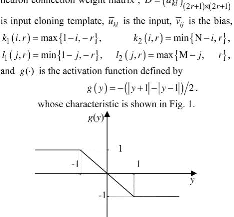
, and g( )⋅ is the activation function defined by

( )

(

1 1 2

)

g y = − y+ − −y . whose characteristic is shown in Fig. 1.

Fig. 1 Piecewise linear function f x t

( )

( ) —negative slope g(y)

y 1

1 -1

(2)

Let r=1 and n= ×N M. If the system (1) has N rows and M columns, then it can be put in vector form as

( )

x= −Cx+Af x +DU+V , (2)

where

(

_{1 2}, , ,

)

T

(

_{11 12, , 1}, , ,

)

T

n M NM

x= x x " x = y y _"y " y , coefficient matrices A andDare obtained through the

templatesAandD, C=diag c

(

₁"c_n

)

, the input vector

(

1,..., n

)

T

U = u u , V =

(

v₁,...,v_n

)

T and

( )

(

( )

1 ,...,

( )

n

)

T

f x = g y g y . The kth cell in Eq. (2) is denoted by Οk(k=iN+ j, where 1≤ ≤i N, 1≤ ≤j M , i denotes ith row and j denotes jth column of the CNN). The matrix A=

( )

aij _{n n}_× , defined by (2), composed of template has the form

1 2

3 1 2

3 1

1 2

3 1

0 0 ... 0 0

0 ... 0 0

0 0 ... 0 0

0 0 0 0 0

0 0 0 0 0 _{n n}

A A

A A A

A A

A A A A _×

⎡ ⎤ ⎢ ⎥ ⎢ ⎥ ⎢ ⎥ ⎢ ⎥ ⎢ ⎥ ⎢ ⎥ ⎢ ⎥ ⎢ ⎥ ⎢ ⎥ ⎣ ⎦ # # # # % # # , 00 01

0, 1 00 01

0, 1 00 1

00 01

0, 1 00

0 0 0

0 0

0 0 0

0 0 0 _{M M}

a a

a a a

a a A a a a a − − − _× ⎡ ⎤ ⎢ ⎥ ⎢ ⎥ ⎢ ⎥ =⎢ ⎥ ⎢ ⎥ ⎢ ⎥ ⎢ ⎥ ⎢ ⎥ ⎣ ⎦ " " " # # # % # # " " , 10 11 1, 1 10 11

1, 1 10 2

10 11 1, 1 10

0 0 0

0 0

0 0 0

M M

a a

a a a

a a A a a a a − − − _× ⎡ ⎤ ⎢ ⎥ ⎢ ⎥ ⎢ ⎥ =⎢ ⎥ ⎢ ⎥ ⎢ ⎥ ⎢ ⎥ ⎢ ⎥ ⎣ ⎦ " " " # # # % # # " " and 1,0 1,1 1, 1 1,0 1,1

1, 1 1,0 3

1,0 1,1

1, 1 1,0

0 0 0

0 0

0 0 0

M M

a a

a a a

a a A a a a a − − − − − − − − − − − − − − _× ⎡ ⎤ ⎢ ⎥ ⎢ ⎥ ⎢ ⎥ =⎢ ⎥ ⎢ ⎥ ⎢ ⎥ ⎢ ⎥ ⎢ ⎥ ⎣ ⎦ " " " # # # % # # " " .

The definition of matricesD

( )

d_{ij n n}

×

= is similar toA.

System (2) can be written as

( )

, 1, ,

i i i ii i i

x = −c x +a f x +w i = " n (3)

where

( )

1, 1

n n

i ij j ij j i

j j i j

w a f x d u v

= ≠ =

=

∑

+

∑

+ . (4)

In Eq. (3), if − ≤1 x ti

_{( )}

≤1 , f x t

(

i

( )

)

= −x ti

( )

. Therefore, when − ≤1 x ti

_{( )}

≤1 , Eq. (3) can be transformed as

( )

(

) ( )

i i ii i i

x t = − c +a x t +w ;

if x ti

_{( )}

≥1, we have f x t

(

i

( )

)

= −1. Therefore, when

( )

1

i

x t ≥ , Eq. (3) can be transformed as

( )

i i i ii i

x t = −c x t −a +w ;

if x ti

_{( )}

≤ −1, we have f x t

(

i

( )

)

=1. Therefore, when

( )

1

i

x t ≤ − , Eq. (3) can be transformed as

( )

i i i ii i

x t = −c x t +a +w.

In Eq. (3), if x ti

_{( )}

=1, we have

( )

1

i i ii i

x t = − −c a +w =R ,

and if x ti

_{( )}

= −1, we have

( )

2

i i ii i

x t = +c a +w =R .

Suppose thatβiis equilibrium point of system (3), then we have

( )

0

i i ii i i

cβ a f β w

− + + = . (5) Whenβi≤ −1 , we have f

( )

βi =1, and the Eq. (5) can be transformed as

(

)

,

i aii wi c ti

β = + ′ → ∞, (6) where

1, 1

n n

i ij ij j i

j j i j

w a d u v

= ≠ =

′ =

∑

± +

∑

+ ; (7)

Whenβi≥1 , we have f

( )

βi = −1, and the Eq. (5) can be transformed as

(

)

,

i aii wi c ti

β = − + ′ → ∞. (8) For simplicity, denote

1

n

i ij j

j d u ρ = =

∑

and 1, n i ij

j j i

a ϑ

= ≠

=

∑

.

Note 1. Let δ be the sum of a cell and the number of its

adjacent cells.

From above analysis about CNNs, we can get the following theorem.

Theorem 1. In Eq. (3), when a_ii< −c_i,

(i) if vi >ρ ϑi+ − −i ci aii, then there exist only positive stable equilibrium points for cell Oi, and the number of these points is grater than or equal to 1 and less than or equal to ₂δ−1_{for cell}

i

O;

(ii) if vi<aii+ −ci ρ ϑi− i, then there exist only negative stable equilibrium points for cell Oi, and the number of these points is grater than or equal to 1 and less than or equal to ₂δ−1_;

(3)

number of stable equilibrium points is greater than or equal to2and less than or equal to 2δ_.

Proof. (i) From a_ii< −c_i, we have R₁>R₂. In terms of

i i i i ii

v >ρ ϑ+ − −c a , we have R₂>0. The x−x phase

plane trajectory of Eq. (1) is shown in Fig. 2.

Fig. 2 The x−x phase plane trajectory of Eq. (3), where R₂>0

and aii< −ci

Therefore there exist positive stable equilibrium points for cell Oi. From Eq. (7) and (8) and R1>0, we know that the equilibrium point of Eq. (3) is

(

)

*

00 i i 1

x = a +w′ c ≥ .

Then, the number of different values of _x*_{is equal to}

that of wi′. If akl =0, for all

( ) ( )

k l, ≠ 0,0 , then the number of different values of wij′ is 1. If akl ≠0, for all

( ) ( )

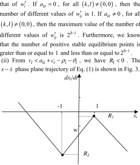
k l, ≠ 0,0 , then the maximum value of the number of different values of wij′ is 2δ−1. Furthermore, we know that the number of positive stable equilibrium points is grater than or equal to 1 and less than or equal to₂δ−1_.

(ii) From vi <aii+ − −ci ρ ϑi i , we have R1<0 . The

x−x phase plane trajectory of Eq. (1) is shown in Fig. 3.

Fig. 3 The x−x phase plane trajectory of Eq. (1), where R1<0 and

ii i

a < −c .

There exist only negative stable equilibrium points for cell Oi, and the number of these points is grater than or equal to 1 and less than or equal to ₂δ−1_.

(iii) From vi ≥aii+ + +ci ϑ ρi i and

i ii i i i

v ≤ − − − −a c ϑ ρ , we have R₁>0 and R₂<0. The

x−x phase plane trajectory of Eq. (1) is shown in Fig. 4.

Fig. 4 The x−x phase plane trajectory of Eq. (1), where R₁>0,

2 0

R < and aii< −ci.

Then, we can get our result.

Corollary 1. In Eq. (6), choose initial statex

( )

0 =0, and

letaii< −ci,

(i) if

0

i i i

v − ρ − ϑ > ,

and

i ii i i i

v ≤ − − − −a c ϑ ρ

then there exist positive stable equilibrium points, and the number of these points is grater than or equal to 1 and less than or equal to ₂δ−1_;

(ii) if

0

i i i

v + ρ + ϑ <

and

i ii i i i

v ≥a + + +c ϑ ρ

then there exist negative stable equilibrium points, and the number of these points is grater than or equal to 1 and less than or equal to ₂δ−1_.

Theorem 2. In Eq. (6), when a_ii= −c_i,

(i) if vi > ρ + ϑi i, then there exists only positive stable equilibrium points for cell Oi, and the number of these points is grater than or equal to 1 and less than or equal to

1

2δ− _;

(ii) if vi< ρ + ϑi i, then there exists only negative stable equilibrium points for cell Oi, and the number of these points is grater than or equal to 1 and less than or equal to

1

2δ− _.

Theorem 3. In Eq. (6), whena_ii> −c_i,

(i) if vi≥ ϑ + ρi i, there exist not more than 2δ−1 positive stable equilibrium points for cell Oi , if

i i ii i i

v ≥ +c a + ϑ + ρ , stable equilibrium points are equal

or greater than 1 for cell Oij;

(ii) if vi ≤ ϑ + ρi i , there exist not more than

1

2δ−

negative stable equilibrium points for cell Oi , if

i i ii i i

v ≤ +c a − ϑ − ρ , stable equilibrium points are equal

or less than -1 for cell Oi. dxi/dt

xi

R1

1 -1

R2

w

dxi/dt

xi

R1

1 -1

R2

w dxi/dt

xi

R1

1 -1

R2

(4)

III. NUMERICAL EXAMPLE

In this section, some numerical simulations are given to verify the theoretical results. Consider a cellular neural network, and its cloning template A is as follows:

1, 1 1,0 1,1 0, 1 00 0,1 1, 1 1,0 1,1

a a a

A a a a

a a a

− − − −

− −

⎛ ⎞

⎜ ⎟

=⎜ ⎟

⎜ ⎟

⎝ ⎠

. (9)

Therefore, a CNN with 2 rows and 2 columns can be written as

( )

(

)

(

( )

)

( )

(

)

(

( )

)

( )

(

)

(

( )

)

( )

(

)

(

( )

)

( )

(

)

(

( )

)

( )

(

)

(

( )

)

11 11 11 00 11 0,1 12 1,0 21 11 22 11 12 12 12 0, 1 11 00 12 1, 1 21 1,0 22 12 21 21 21 1,0 11 1,1 12

00 21 0,1 22 21 22

,

x c x a f x t a f x t

a f x t a f x t

x c x a f x t a f x t

a f x t a f x t

x c x a f x t a f x t

a f x t a f x t

x

−

− −

= − + +

+ + + η

= − + +

+ + + η

= − + +

+ + + η

=

(

( )

)

(

( )

)

( )

(

)

(

( )

)

22 22 1, 1 11 1,0 12 0. 1 21 00 22 22,

c x a f x t a f x t

a f x t a f x t

− − −

−

⎧ ⎪ ⎪ ⎪ ⎪ ⎪ ⎪⎪ ⎨ ⎪ ⎪ ⎪ ⎪

− + +

⎪

⎪₊ ₊ _{+ η}

⎪⎩

where

11 00 11 0,1 12 1,0 21 11 22 11 12 0, 1 11 00 12 1, 1 21 1,0 22 12

21 1,0 11 1,1 12 00 21 0,1 22 21 22 1, 1 11 1,0 12 0. 1 21 00 22 22

, , ,

.

d u d u d u d u v

d u d u d u d u v

d u d u d u d u v

d u d u d u d u v

− −

− − − −

η = + + + +

⎧ ⎪

η = + + + +

⎪ ⎨

η = + + + +

⎪

⎪_{η =} ₊ ₊ ₊ ₊

⎩

In Fig. 5 (a) and (b), inputs and outputs of CNNs are shown, respectively, where the white lattice stands for -1 and black for 1.

Fig. 5 Inputs of CNNs are shown in (a), and outputs are shown in (b).

We are based on Corollary 1 to design a CNN. Choose

0.5 0.3 0.1

0.1 5.9 0.1

0.2 0.4 0.1

A

− − −

⎛ ⎞

⎜ ⎟

=_⎜ − _⎟

⎜ ⎟

⎝ ⎠

, c11= =c12 c21=c22=1, and

0.3 0.1 0.1

0.2 0.2 0.2

0.2 0.4 0.1

D

− −

⎛ ⎞

⎜ ⎟

=_⎜ _⎟

⎜ ₋ ⎟

⎝ ⎠

.

Then, from inputs and outputs of CNNs in Fig. 6, we can get

11 12

2.3<v <2.6, − 2.6 <v < −2.3,

21 1.3, 1.7 22 3.2

v v

−3.6 < < − < < . Therefore , we choose

11 2.5, 12 2.4, 21 3, 22 3

v = v = − v = − v = .

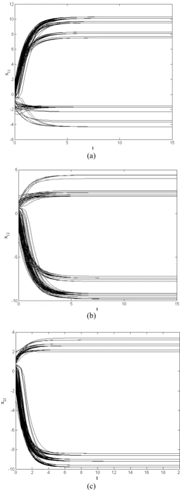
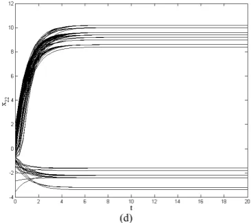
Furthermore, a CNN is obtained. Fig. 6 shows the number of equilibrium points, where all parameters of the CNN are based on Corollary 1 (iii), and 100 random

initial states are used. We can find that the number of equilibrium points is accord with Corollary 1.

IV. CONCLUSIONS

In the paper, the region of the number of equilibrium points of cellular neural networks was considered by the relationship between parameters of cellular neural networks with negative slope activation function. We find that there are no more than 3δ_{isolated equilibrium points}

or 2δ_{equilibrium points located in saturation regions for}

a cell in a CNN. Finally, numerical simulations were presented to verify the theoretical results.

(a)

(b)

(5)

(d)

Fig. 6 The number of equilibrium points of every cell CNNs are shown,

where the number of different equilibrium points of every cell can be known.

ACKNOWLEDGMENT

This work was supported in part by Research Project of Chongqing University of Science and Technology(CK2013B15, CK2011Z17), in part by Teaching & Research Program of Chongqing Education Committee (KJ131401, KJ131416, KJ121505, KJzh11221), in part by the National Natural Science Foundation of China (61170249, 61003247), in part by the Natural Science Foundation project of CQCSTC ( cstc2011pt-gc70007, 2010BB2284, cstc2011jjA80022, cstc2011jjA40005, and in part by the First Batch of Supporting Program for University Excellent Talents in Chongqing.

REFERENCES

[1] L. O. Chua and L. Yang, Cellular neural networks: theory, IEEE Transactions Circuits Systems, 35:1257-1272, 1988. [2] L. O. Chua and L. Yang, Cellular neural networks:

applications, IEEE Transactions Circuits Systems, 35:1273-1290 1988.

[3] M. Itoh, L.O. Chua, Advanced image processing cellular neural networks, International Journal of Bifurcation and Chaos, 17: 1109-1150, 2007.

[4] Z. G. Zeng, and J. Wang, Associative memories based on continuous-time cellular neural networks designed using space-invariant cloning templates, Neural Networks, 22: 651-657, 2009.

[5] L. O. Chua and T. Roska, Cellular neural networks and visual computing, Cambridge: Cambridge University Press, 2002.

[6] S. P. Xiao and X. M. Zhang, New globally asymptotic stability criteria for delayed cellular neural networks, IEEE Transactions on Circuits and Systems—II: Express Briefs, 56: 659-663, 2009.

[7] C. J. Li, C. D. Li, X. F. Liao and T. W. Huang, Impulsive effects on stability of high-order BAM neural networks with time delays, Neurocomputing, 74: 1541-1550, 2011. [8] Q. Han, X. Liao, T. Weng, C. Li and H. Huang, Analysis

on equilibrium points of cells in cellular neural networks described using cloning templates, Neurocomputing, 89: 106-113, 2012.

[9] Q. Han, X. Liao, T. Weng, C. Li and Hongyu Huang, Analysis on equilibrium points of cellular neural networks

with thresholding activation function, Neural computing & Applications, Published online: 26 September 2012. [10]Q. Han, X. Liao and C. Li. Analysis of associative

memories based on stability of cellular neural networks with time delay. Neural Computing & Applications, Published online: 20 January 2012.

[11]Q. Han, X. Liao, T. Huang, J. Peng, C. Li and H. Huang. Analysis and design of associative memories based on stability of cellular neural networks. Neurocomputing, 97: 192-200, 2012.

Qi Han received the B.S. degree in

Computer Science and Technology from Shandong University (Weihai), China, in 2005. He received M.S. degree in Computer Software and Theory from Chongqing University, China, in 2009. He received PhD degree in Computer Science and Technology at Chongqing University of China in 2012. Now he is a Lecturer with School of Electrical and Information Engineering, Chongqing University of Science and Technology. His current research interest covers chaos control and synchronization, cellular automata, neural network, associative memories.

Qian Xiong received the B.S. degree and

the M.S. degree in computer science from Chongqing University, Chongqing, China, in 2003 and 2006 respectively. She is currently a Lecturer with the School of Electrical and Information Engineering, Chongqing University of Science and Technology. Her research interests include artificial intelligence, web application and bilingual teaching.

Chao Liu received his Ph. D degree from Chongqing

Universtiy in 2012. Now he is a Lecturer with School of Electrical and Information Engineering, Chongqing University of Science and Technology, People's Republic of China. His current research interests include impulsive systems, switched systems and neural networks.

Jun Peng is a professor with School of Electrical and

Information Engineering, Chongqing University of Science and Technology.

Lepeng Song is professor with School of Electrical and

Information Engineering, Chongqing University of Science and Technology.

Sijing Liu is assistant with School of Electrical and Information