Analysis of Average Shortest-Path Length of Scale-Free Network with Secure Routing

ISSN (e): 2250-3021, ISSN (p): 2278-8719

Vol. 09, Issue 5 (May. 2019), ||S (II) || PP 20-27

−

−

Analysis of Average Shortest-Path Length of Scale-Free Network

with Secure Routing

G.Prathyusha

1

,V. Jaikumar

2

1

PG Student(DECS),Department of ECE,QIS College of Engineering and Technology,Ongole, 2_{Associate Professor, Department of ECE,QIS College of Engineering and Technology,Ongole,AP-523272}

Corresponding Author:G.Prathyusha

Abstract: Computing the average shortest-path length of a large scale-free network needs much memory space

and computation time. Hence, parallel computing must be applied. In order to solve the load-balancing problem for coarse-grained parallelization, the relationship between the computing time of a single-source shortest-path length of node and the features of node is studied. We present a dynamic programming model using the average out degree of neighboring nodes of different levels as the variable and the minimum time difference as the target. The coefficients are determined on time measurable networks. A native array and multimap representation of network are presented to reduce the memory consumption of the network such that large networks can still be loaded into the memory of each computing core. The simplified load-balancing model is applied on a network of tens of millions of nodes. Our experiment shows that this model can solve the load-imbalance problem of large scale-free network very well. Also, the characteristic of this model can meet the requirements of networks with ever-increasing complexity and scale.

Keywords: Shortest Path, scale free Network, Secure Routing, Network Simulator.

--- --- Date of Submission: 09-05-2019 Date of acceptance: 25-05-2019

---

I.

INTRODUCTION

A complex dynamic system is constituted by many elements that interact among themselves and with the environment. Recently, connection networks have been described, studied, characterized and represented by parameters using concepts of Complex Systems domain. These networks may be natural such as the neuron system of the human brain, the chemic molecular connections in protein conglomerates, the system of virus propagation in an epidemic situation etc. Or artificial, such as the lines of energy distribution in a country, the tangled social contacts that we make through our lives or the Internet, which is one of the most interesting examples and certainly the most modern one [4][6][10].

The Internet may be seen under several levels of reach and complexity considering different basic units. The most intuitive view and of easy understanding to the general public, is to suppose that these units are computers connected by wires, optical fibers or even using wireless technology through the whole planet. An- other vision, a little bit wider, defines basic unit as a cluster of computers, servers, printers, switchers and routers which form a Local Area Network LAN. Each institution, company or residential building, would have its LAN which would be connected to others LANs and so on.

A third vision would be to consider the Internet basic element as an Autonomous System AS. A straight definition would be: an AS is defined as a cluster of LANs or routers submitted to the same policy of usage, connectivity and technically administrated by the same network management group.

Each ASs registered at a regional control organism receives a number ASN be- tween 1 and 65536 that will be a digital print to the whole Internet and will be used to configure the routers. The IP prefixes of LANs‟ addresses of an AS are represented by one ASN. The number of autonomous systems increases in a daily basis, in 1998 there were around 2550 and nowadays about 21000 ASNs are used. AS numbers are not contiguous because some are reserved, others dedicated and some are no longer used due end of operation.

τ n

from 1998 to 2007 and the shortest path length (L), obtained by a proposed computational method (Friburgo algorithm) among each pair of ASs represented in the adjacency matrix.

II.

RELATED WORK

The concept of patient monitoring system is explained in the paper “Implementation of wireless body area networks for healthcare system,” The concept of Ad-hoc network for patient The patient monitoring is implemented in “ Real time monitoring of electrocardiogram through IEEE 802.15.4 network” under IEEE standard of WPAN and real time monitoring is explained by monitoring system is explained by PoraminInsomet al in his paper “Implementation of a human vital monitoring system using Ad Hoc wireless network for smart healthcare”.The routing is core issue for mobile patient system and the routing algorithm is discussed in the paper The performance evaluation of different routing protocol in his paper “A simulation comparison among SCALE FREE , DSDV, DSR protocol with IEEE 802.11 MAC for grid topology in MANET” It states that thescale free routing is reactive On demand routing protocol. DSR routing protocols explained in paper “Optimization and implementation of DSR route protocol based on Ad hoc network” , the threshold value of onset of small- world behavior has been determined as, limn→∞logp= −1 . This result leaves a wide range of p values where we cannot decide whether the network is smallor not, i.e., when τ = 1. In this work, we use Erdős-Rényi random networks which have the advantage of being analytically solvable in many of their aver- age properties and being one of the oldest and best studied network models, to construct a solvable small-world network model. Using random network structure R(n, p) when np is bounded away from zero, we narrow the threshold to be p = εwhere ε is a constant ε >0, and we construct a small-worldnetwork with diameter (log n) which bounds the average path length below by (log n). In addition, we study the random network structure when pntends to zero, and we use the result to study average path length of small- world models. We show that in this case ¯l >(log n), i.e., the network is not small-world. We deduce that at least εnwhere ε is a constant and ε >0 random links should be added to a one dimensional lattice to ensure average path length of order log n.In addition to the analytical work, we conduct an empirical study of the scientific collaboration, citation and Facebook social network data by analyzing their average path lengths, clustering and degree distributions. The results show the unsuitability of random networks as models of real-world networks, as they do a poor job of capturing real-real-world network properties like the high clustering and the scale-free degree distribution. In addition, we simulate Watts and Strogatz (1998) and Newman and Watts (1999a) models of small- world networks to confirm the results and to compare their properties with real-world network properties. Small-world network models do a good job in capturing real-world network properties but they do not have the scale-free degree distribution. However, it should be noted that the models were never intended to mimic real-world degree distribution.

III.

SHORTEST PATH LENGTH

This section presents a proposed algorithm to compute the Shortest Path Length −L, introducing the features of the method and the dynamic used.

Figure 1: Log Log plot of the rank evolution of connectivity degree ki. The legend shows the annual evolution of the angular coefficients a of the log log linear adjustments of the curves.

Shortest Path Calculation

Theory, the shortest path problem is the problem of finding the way between two vertices or nodes, that the sum of the connections weight is minimized. The average L used in this work is the mean of all shortest paths between each AS with all others.

The L parameter calculation is a classic problem studied by several authors that developed its own algorithms. Each one has its own importance and performance, being appropriate when some features are present, e.g. Dijkstra [10] for non-negative connection weights, and Bellman [5] and Ford independently for negative and positive weights, Dantzig et. al. [9] for sparse graphs, etc.

In the case of the complex network of the Internet ASs connections, all weights are defined as “1” and, for this reason, one start the method with the Dijkstra algorithm, where the temporal complexity is O(N 2) with N meaning the number of nodes in the network.

The characteristicsof the program developed byEscard´o imposed restrictions for its utilization in this work. In a 64 bits High Performance Computing System - HPCS, the execution time for the smaller connection networks of ASs for the year 1998 (concerning 2,500 ASs) were greater than 8 days and for more recent years, we compute for more than 30 days without a final result.

Figure 2: Diagram of the shortest path length calculating algorithm

Moreover the computing restrictions to calculate bigger networks (around 21,000 ASs in 2007) required the development of a new algorithm adapted for our needs and for our computing resources. The new algorithm was named Friburgo Method because of the city where it was conceived. To understand it, lets consider a practical example:

Consider a connection network composed of 6 connected nodes as shown in figure An edge is represented by a bidirectional connection: (A,B), (A,D), (A,E), (B,E),

(B,F) and (C,F). This figure also shows the adjacency matrix - AM of this example network. The method requires a repetitive procedure for each node or matrix line. In each line of the AM an X character represents a node and the symbols „1‟ and „0‟ represent the existence, or not, of a connection between them respectively. The basic concept of the proposed method is to search missing connections in the AM lines on those points where a direct connection between nodes already exists. For example, starting from node A the algorithm search for connections with C and F only in B, D and E node lines. If we observe node B line, there exist three connections (B,A), (B,E) and (B,F). The first two are not considered, because node A is already connected to itself and to node E. The connection (B,F) indicates an indirect connection (A,B,F) considered as a level 2 one. Assuming this same procedure for nodes D and E one can easy observe any new level 2 connection. We have still a missing indirect connection (A,...,C) represented by the 0 in the second line of the scheme of node A. The process is repeated up to node F line observing two connections (two symbols „1‟) in it. The (F,B) edge doesn‟t add any new information to the algorithm but (F,C) edge is part of (A,B,F,C) path, which is a level 3 one because it came from the level 2 path (A,B,F) which, for its turn, came from the initial edge (A,B), level 1. Finally, we do not have any more connections and the algorithm passes to next node, B. In this case, the searching for indirect connections of node B to nodes C and D can be seen in lines of nodes F and A, respectively. Both are connections of level 2 to the algorithm.

IV.

METHODOLOGY

NETWORK SIMULATOR (NS)

networks. The simulator is a result of an ongoing effort of research and developed. Even though there is a considerable confidence in NS, it is not a polished product yet and bugs are being discovered and corrected continuously.

NS is written in C++, with an OTcl1 interpreter as a command and configuration interface. The C++ part, which is fast to run but slower to change, is used for detailed protocol implementation. The OTcl part, on the other hand, which runs much slower but can be changed very fast

quickly, is used for simulation configuration. One of the advantages of this split-language program approach is that it allows for fast generation of large scenarios. To simply use the simulator, it is sufficient to know

OTcl. On the other hand, one disadvantage is that modifying and extending the simulator requires programming and debugging in both languages.

NS can simulate the following: 1. Topology: Wired, wireless

2. Sheduling Algorithms: RED, Drop Tail, 3. Transport Protocols: TCP, UDP 4. Routing: Static and dynamic routing

5. Application: FTP, HTTP, Telnet, Traffic generators

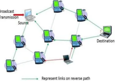
Fig 3. Route discovery process RREQ broadcast

ROUTE DISCOVERY PROCESS RREP

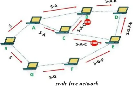
scale free network

Fig 4. Scale free NETWORK

shows that if source node after checking in routing cache found that route to the destination are not there, and then source node broadcast RREQ in the network shown by red arrow in the network.

Fig 5. Scale free RREQ MESSAGE PROCESSING

RREQ message contains the IP address of source and intended node with the current sequence number of source and last known sequence number of destination. In figure 2-6, it is shown that whenever any in between node receive the route request, it first check whether that request came earlier or not. If the same request came before, intermediate node will discard that request. Each node setup a reverse link and route entry in routing table. The process of forwarding RREQ is continued until it reaches the intended node for packet sent by source node that process

Fig 6. SCALE FREE REVERSE PATH SETUP

Destination node will not forward the RREQ message further in the network because the destination node is the intended target for the original packet of information being sent by source node. Each node forms a reverse path to source from it, and update in routing protocol.

V.

PROPOSED METHODOLOGY

We are presenting the improved method for SFN routing protocol with aim of improving energy efficiency of SFN network as compared to existing routing protocols. Here we added the new energy efficient function in existingscale free routing protocol. Here we have taken two routing protocols under investigation such as SCALE FREE , DSR and the modifiedscale free routing protocol. Following is the algorithm which is added to thisscale free routing protocol for the improvement of energy and hence the other parameters. For a packet P, we use hc(P) and lvl(P) to represent the two additional fields of the packet, respectively. The algorithm needs to access other fields in a packet, such as the source, destination, sender and sequence number. Similarly, in the algorithm, they are represented by s(P), d(P), nid(P) and seq(P). We use s-d (P) to represent the source-destination pair of the flow that the packet belongs to. An “overhear table” is maintained at each node.

Algorithm: When node i overhears packet P,BEGIN Step 1: Lookup s-d (P) in overhear table;

Step 2: IF no match, add entry e‟: s-d(e‟)=s-d(P), seq(e‟)=seq(P),ov-list(e‟) initialized with first entry <hc(P),lvl(P),nid(P)>. GOTO END;

Step 3: (Assume a match is found at entry e.) IF seq(P)<seq(e),ignore P. GOTO END;

Step 4: IF seq(P)>seq(e), update e as the following:seq(e)=seq(P), ovlist(e) reset as having only one entry <hc(P),lvl(P),nid(P)>. GOTO END;

Step 5: IF seq(P)==seq(e), do the following:

Step 5.1: Add entry <hc(P),lvl(P),nid(P)> into ovlist(e);

Step 5.2: IF ovlist(e) has three entries A, B, C satisfying thefollowing conditions, a better sub-path is found. 1)hc(C)==hc(B)+1==hc(A)+2;

2)lvl(node i)≥MAX(lvl(A),lvl(C));

3) (lvl(node i) -lvl(B))≥2. Activate this new subpath. Delete entry e from overhear table. GOTO END;

Step 5.3: IF ovlist(e) has two entries A and B, such thathc(B)==hc(A)+1 and lvl(node i) ≥ MAX(lvl(A),lvl(B)+2), add this indicator I in the WaitingIndicator list: candidate(I)=B, seq(I)=seq(e), s-d(I)=s-d(e). GOTO END;

Step 5.4: IF ovlist(e) has two entries B and C, such thathc(C)==hc(B)+1 and lvl(node i) ≤ MAX(lvl(B)+2,lvl(C)), node i broadcast one SHORT informing packet Q as follows: candidate(Q)=B, seq(Q)=seq(e) s-d(Q)=s-d(e); When node i receives a SHORT informing packet Q, BEGIN

1. Compare fields of Q with any valid entry in Waiting Indicator list;

IF there is no match, ignore packet Q; ELSE a better subpath is found

VI.

CONCLUSION

In this chapter three topics have been discussed. Firstly, we introduced com- plex network terminologies by defining three important properties that are used to characterize complex networks. We then described random networks and their properties. Finally, we investigated three examples of real-world net- works and compared their properties with random networks. The comparison showed that Erdős and Rényi random networks do a poor job as a model of real-world networks.

The three metrics in question are: the average path length, the clustering coefficient and the degree distribution. The importance of these quantities has been emphasised by empirical studies of real-world networks which have recently revived network modelling and resulted in an enormous number of studies in network science. First, random networks: despite the fact that their properties deviate from real-world networks, random networks are still widely used in many fields and serve as a standard for many modelling and empir- ical studies. In addition there are many studies devoted to overcoming the shortcoming of random networks as a model of real-world networks; see (New- man, 2003a; Newman et al., 2002). Second, stimulated by the high clustering property observed in real-world networks, a class of models called small-world models has been proposed which interpolate between the high clustering reg- ular lattices and random networks (Watts and Strogatz, 1998). Finally, the discovery of the power-law degree distribution has led to the construction of various scale-free models (Barabási and Albert, 1999) (not part of this study).

REFERENCES

[1]. I. Paik, T. Tanaka, H. Ohashi and W. Chen, “Big Data Infrastructure for Active Situation Awareness on

Social Network Services,” Big Data (BigData Congress), 2013 IEEE International Congress on. IEEE, pp. 411-412, 2013.

[2]. E. Hargittai, “Is Bigger Always Better? Potential Biases of Big Data Derived from Social Network Sites,” Annals of the American Academy of Political & Social Science, vol. 659, no. 1, pp. 63-76, 2015.

International organization of Scientific Research

27 | Page

[4]. I. Hashem, I. Yaqoob, N. Anuar, et al., “The rise of “big data” on cloud computing: Review and open

research issues,” Information Systems, vol. 47, no. 47, pp. 98-115, 2015.

[5]. H. Li, Y. Yang, T. Luan, X. Liang, L. Zhou and X. Shen, “Enabling Fine grained Multi-keyword Search

Supporting Classified Sub-dictionaries over Encrypted Cloud Data,” IEEE Transactions on Dependable and Secure Computing, DOI10.1109/TDSC.2015.2406704, 2015.

[6]. H. Li, D. Liu, Y. Dai and T. Luan, “Engineering Searchable Encryption of Mobile Cloud Networks: When QoE Meets QoP,” IEEE WirelessCommunications, vol. 22, no. 4, pp. 74-80, 2015.

[7]. X. Liu, B. Qin, R. Deng, Y. Li, “An Efficient Privacy-Preserving Out-sourced Computation over Public

Data,” IEEE Transactions on Services Computing, 2015, doi: 10.1109/TSC.2015.2511008

[8]. X. Liu, R. Choo, R. Deng, R. Lu, “Efficient and privacy-preserving out-sourced calculation of rational

numbers,” IEEE Transactions on Depend-able and Secure Computing, 2016, doi:

10.1109/TDSC.2016.2536601.

[9]. H. Li, X. Lin, H. Yang, X. Liang, R. Lu, and X. Shen, “EPPDR: An Efficient Privacy-Preserving Demand Response Scheme with Adaptive Key Evolution in Smart Grid,” IEEE Transactions on Parallel and Distributed Systems, vol. 25, no.8, pp. 2053-2064, 2014.

[10]. H. Li, R. Lu, L. Zhou, B. Yang, X. Shen, “An Efficient Merkle Tree Based Authentication Scheme for

Smart Grid,” IEEE SYSTEMS Journal, vol. 8, no.2, pp. 655-663, 2014.

G.Prathyusha. “Analysis of Average Shortest-Path Length of Scale-Free Network with Secure

Routing.” IOSR Journal of Engineering (IOSRJEN), vol. 09, no. 05, 2019, pp. 20-27.