R E S E A R C H
Open Access
Cloud computing and its interest in saving
energy: the use case of a private cloud
Robert Basmadjian
1*, Hermann De Meer
1, Ricardo Lent
2and Giovanni Giuliani
3Abstract
Background: Cloud computing data centres, due to their housing of powerful ICT equipment, are high energy consumers and therefore accountable for large quantities of emissions. Therefore, energy saving strategies applicable to such data centres are a very promising research direction both from the economical and environmental stand point. Results: In this paper, we study the case of private cloud computing environments from the perspective of energy saving incentives. However, the proposed approach can also be applied to any computing style: cloud (both public and private), traditional and supercomputing. To this end, we provide a generic conceptual description for ICT resources of a data centre and identify their corresponding energy-related attributes. Furthermore, we give power consumption prediction models for servers, storage devices and network equipment. We show that by applying appropriate energy optimisation policies guided through accurate power consumption prediction models, it is possible to save about 20% of energy consumption when typical single-site private cloud data centres are considered. Conclusion: Minimising the data centre’s energy consumption, on one hand acknowledges the potential of ICT for saving energy across many segments of the economy, on the other hand helps ICT sector to show the way for the rest of the economy by reducing its own carbon footprint. In this paper, we show that it is possible to save energy by studying the case of a single-site private cloud data centres. We believe that through the federation of several cloud data centres (both private and public), it is possible to minimise both the energy consumption as well as CO2emissions.
Keywords: Private cloud computing data centre, Modelling, IT resources, Power and energy consumption
Background Motivation
Energy consumption of data centres is becoming a key concern for their owners:energy costs(fuel) continue to rise and CO2 emissions related to this consumption are relevant. In 2007, Gartner [1] estimated that the global impact of the ICT sector (considering PCs, servers, cool-ing, fixed and mobile telephony, local area network, office telecommunications and printers) is 2% of the global CO2 emissions, which is approximately the same as fuel con-sumption from the airline industry.
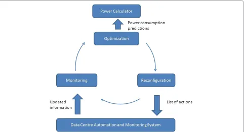
Amazon [2] has evaluated its data centre expenses (see Figure 1), showing that server costs account for 53%, while energy related costs totaling 42% (direct power consump-tion 19% plus amortised power and cooling infrastructure 23%).
*Correspondence: [email protected] 1University of Passau, Innstrasse 43, 94032 Passau, Germany Full list of author information is available at the end of the article
Therefore, saving money in the energy budget of a data centre, without sacrificing Service Level Agreements (SLA) is an excellent incentive for data centre owners, and would at the same time be a great success for environ-mental sustainability. This aspect needs to be highlighted, since it’s absolutely not frequent in environment-related problems to have a solution satisfying all stake holders.
Main focus
One of the latest trends in IT is cloud computing [3], where public and private deployment models [4] are commonly used to differentiate one cloud provider from another. The former is made available to the general public on pay-per-use basis, whereas the latter is operated solely for internal users of organisations.
Sinceelasticity [4] is one of the key aspects of a cloud service, the cloud provider gives the impression of hav-ing an infinite set of resources. In fact, large public cloud providers have end users potentially spread over the globe
Figure 1Amazon’s monthly expenses distribution.Amazon’s evaluation of its data centre expenses showing that server costs account for 53%, while energy related costs totaling 42%.
and can capitalise on statistical compensation for large number of service requests; practically speaking, since cloud resources are frequently allocated and also released (as side effect of the pay-per-use billing mode), during the time lots of allocations and de-allocations tend to com-pensate keeping fluctuations under reasonable control. On the other hand, private clouds, instead, have generally a much smaller number of users (e.g. the employees of a corporation) and the provider needs to size its ICT infras-tructure for the peak usage. Since the variety of usage patterns is limited inside a close community, it’s quite likely that the utilisation rate of the ICT resources can vary a lot between night and day and/or week days and week-ends. Therefore, private cloud providers need to keep a larger capacity buffer compared to public providers, and suffer more from load variations. In addition, it has been noticed that some public cloud providers are starting to offer discounted prices for certain time slots, when they foresee a resource usage gap – something similar to the concept of “last minute” tickets for travellers – where private providers don’t have this chance!
Given the above-mentioned differences in the ICT resources’ utilisation patterns between private and public cloud providers, it is obvious that more evident advan-tages are foreseen to save energy in former than in latter where the owners – in case of low load – instead of saving energy and costs, can decide to attract additional business by lowering the prices to fill the utilisation gap. Private cloud provider – in case of low load – has the possibility to see the whole infrastructure optimised to run the load with the lowest energy consumption, while preserving the SLAs with respect to their users.
In summary, there are lots of incentives for any cloud provider – being public or private – to save energy. The opportunities for public cloud providers might depend
on alternative business conducts, while private cloud providers will likely get clear benefits.
Contributions and results
In general, energy savings can be achieved in data centres through optimisation mechanisms whose main objective is to minimise the energy consumption. However, in order that these optimisation mechanisms can take the most suitable energy-saving decisions, the existence of accurate power consumption prediction models becomes primordial. Consequently, one of the major contributions of this paper is devoted to a detailed description of power consumption prediction models for ICT resources of data centres which are presented in Section Power con-sumption prediction models. Note that the details on the optimisation algorithms used for our use-case study are out of the scope of this paper and interested readers can refer to [5].
The architecture of our energy-saving mechanism is based on a three-step control loop: Optimisation, Recon-figuration and Monitoring. The whole state of the data centre is continuously monitored. As a matter of fact, another major contribution of this paper is dedicated to a detailed description of the state of a data centre in terms of ICT resources with their relevant energy-related attributes and interconnections which is introduced in Section Data centre schema. This state is periodically examined by the Optimisation module in order to find alternative software application and services deployment configurations that allow saving energy. Once a suitable energy-saving configuration is detected, the loop is closed by issuing a set of actions on the data centre to reconfigure the deployment to this energy-saving setup.
Monitoring and Reconfiguration modules in Figure 2 interact with the data centre monitoring and automation frameworks to perform their tasks. The Optimisation module ranks the candidate target configurations, identi-fied by applying energy-saving policies without violating existing SLAs, with respect to their power consumption that are predicted by thePower Calculatormodule. The accuracy of the predictions of this module is crucial to take the most appropriate energy-saving decisions; in fact it has the responsibility to forecast the power con-sumption of a data centreaftera possible reconfiguration option. In the rest of this paper, our energy-saving mecha-nism is called “plug-in” simply because it runs agnostically on top of data centres’ automation and monitoring frameworks.
Figure 2Proposed control loop for energy optimisation.The different components and their interactions of our energy-aware “plug-in”. We call it “plug-in” simply because such a set of software components run agnostically on top of data centre automation and monitoring frameworks.
worthwhile to note that our power consumption predic-tion models as well as state descrippredic-tion of a data centre are generic enough that they are suitable to energy-saving optimisation mechanisms applicable to any computing style being traditional, super and cloud computing.
Related work Servers
In the existing literature, the power consumption of a server has been modelled in two different ways:offlineand online. In the former case, SimplePower [6], SoftwareWatt [7] and Mambo [8] estimate the power consumption of an entire server. However, these models use analytical meth-ods based on some low-level information such as number of used CPU cycles. The major advantage is that they provide high accuracy. Nevertheless, the offline nature of such models requires extensive simulation, which results in a significant amount of time for estimating the power consumption. Consequently, these models are infeasible for predicting the power consumption of highly dynamic environments like cloud computing data centres.
To overcome this problem, an online (run-time) methodology is proposed [9,10]. Such models are based on the information monitored through performance counters [11]. These counters keep track of activities performed by applications such as amount of accesses (e.g. to caches) and switching activities within processors. The total power dissipation of a server is computed as
the power consumption of each activity. However, these counters in certain processors (e.g. AMD Opteron) can report only four out of 84 events [12]. Therefore, such models are unable to predict accurate power consumption in real-life cases.
designs different models for different components based on their behaviours. Another distinguishing property is that our approach does not need calibration phase.
It is worthwhile to note that above mentioned approaches, which depend on low-level information in order to predict the power consumption, are not appro-priate in real-life case simply because the underlying monitoring systems of the data centres are not able to provide the low-level information that these approaches require. Consequently, in this paper we identified the most-relevant energy-related attributes of ICT resources to which the monitoring systems of data centres typically provide the necessary information.
Storage devices
The storage devices range from a single hard disk to SAN (Storage Area Network) devices, which consume a signif-icant amount of power. Several studies [15-18] were ded-icated to devise models for individual hard disks, where the power consumption of a disk is predicted based on its states such as seek, rotation, reads, writes and idle. With the emergence of Disk arrays (e.g. RAID), the above mentioned approaches need to be adapted to deal with several hard disks instead of one. Several models [19-21] for RAID have been proposed. [19] proposed STAMP (Storage Modeling for Power) by mapping the front-end workload to back-end disk activities, and the power con-sumption of the back-end activities is computed. A major concern is that this model ignores the power of some activities such as spin-up and spin-down [21]. [20] gener-alised the model of individual hard disks to RAID where the overall power of RAID is the sum of power consumed by each individual hard disk within RAID. However, this model does not take into account the power of RAID controller’s processor and memory. [21] addressed this problem by proposing a model (MIND), which computes the power of RAID by considering controller’s power and disk activities such as idle, sleep, random, sequential and cache accesses.
The key drawback of these RAID models is their imple-mentation in the real world such as data centres due to the low level input parameters. For instance, hard disk’s state (e.g. idle, accessing, startup) and operation mode (read/write operations) are usually not available at data centre level, where a monitoring system provide informa-tion only about average read and write rates over a time period (e.g. per second). Furthermore, the total power consumption of SAN devices, which are used for storage within data centres, cannot be computed through RAID models since SAN has also processing (e.g. CPU, RAM) and network components (I/O ports) in addition to hard disks. In this paper, we propose a model, which can be applied to any type of storage devices. In contrast to the existing models, our approach requires information such
as read/write rate, which is usually available within data centres monitoring systems.
Network equipment
There has been a great deal of attention to devise power consumption models for routers and switch fab-rics. The power consumption of the integrated Alpha 21364 router and the IBM InfiniBand 8-port 12X switch is modelled in [22] illustrating that buffers are the largest power hoggers in routers. A crossbar switch, if present, consumes less but still significant power, and arbiter power is negligible under high network load. It is shown, that also the router micro-architecture has a huge impact on router power consumption. [23] sug-gest a framework to estimate the power consumption on switch fabrics in network routers. They state that the power consumption on switch fabrics is mainly determined by the internal node switches, the inter-nal buffer queues and the interconnect wires. [24] present a power and area model according to network-on-chip architectures. They suggest ORION 2.0 that uses a set of architectural power models for network routers to perform early-stage network-on-chip power estimation.
Data centre schema
The ICT resources (e.g. servers, storage devices and network equipment) with their relevant energy-related attributes and interconnections are represented by the data centre schema. The data centre operator identifies all the equipment that the site is composed of and becomes responsible for creating and editing an instance of such a schema. Note that some forms of automated discovery of resources and exporting them to theschema instance might be provided, however the data centre operators are responsible for validating their configuration.
Given the complexity and heterogeneity of the data cen-tre infrastructure, we derive the data centre schema by decomposing the modelling process into 5 phases: ICT resources, network topology, server, storage, and services modelling.
ICT resources modelling
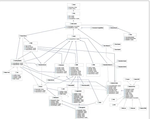
Figure 3ICT resources UML class diagram.The figure, which is a Unified Modeling Language design, describes in detail the different ICT resources that can be found inside a site consisting of several data centres.
paper). Each “Data centre” is based on a specific comput-ing style indicated through the computingStyleattribute which belongs to one of the following three categories: Traditional computing, Supercomputing and Cloud com-puting. Note that the corresponding attribute is useful in order to enable the optimisation policies suitable to each computing style.
Inside each data centre, there are ICT equipment which can be organised either inside “Rack”s or in indepen-dent cases such as single box stands, generally with tower form factor (“Tower Server”), in addition to box-like network devices such as routers and switches (“Box Network” class). “Framework Capabilities” class describes energy-related controlling capabilities of the manage-ment and automation tools available to the data cen-tre to be managed energy-wise. The term controlling capabilities refers to all possible actions (e.g. power off/on equipment, migrate software load, etc.) applied
to the data centre ICT resources and carried through by the framework. As a matter of fact, in the rest of this paper frameworkID attribute is used by every class that needs to identify its corresponding controlling capabilities.
devices simply used to connect the different power plugs of the rack elements; in some other cases they can also be active and perform power measurements and switch on/off functions. Storage Area Network devices (“SAN” class) are generally mounted inside racks and have inde-pendent Power Supply Units and cooling system. SAN is a dedicated device that provides network access to consol-idated, block level storage. Finally, network devices such as routers and switches can also be mounted inside racks (“Rackable Network” class) whose specifics are explained in Section Network topology modelling. Note that in the rest of this paper measuredPower and computedPower optional attributes in most of the classes are used in order to record the power consumption of the correspond-ing resource obtained respectively through a dedicated power meter and power consumption prediction models of Section Power consumption prediction models. These two parameters serve for the model refinement as they are useful to compare measured and computed values to check and refine the power consumption prediction mod-els. Finally,powerIdleandpowerMaxare respectively used to denote the idle and the fully active power consumption of the corresponding class.
Network topology modelling
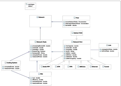
Figure 4 illustrates the network topology UML class dia-gram which depicts a clearer overview of how network nodes in a data centre are connected to each other. A class “Network” consists of number of entities of “Net-work Node” and “Flow”. Flows are allocated to the various nodes based on the network decisions. These allocations are dynamic and can vary during the lifetime of a flow to optimise the energy consumption accordingly. Therefore, the two defined entities of “Network Node” and “Flow” shape the “Network” so that based on certain criteria a “Flow” can be detached from one “Network Node” and can be attached to another. The energy efficient policies that make such decisions are performed based on the attributes from both classes of “Flow” and “Network Node”, which will be elaborated further in the followings.
As illustrated, the “Flow” class describes an end-to-end communication occurring within the data centre or between one network node within the data centre and another node on an external network (for example the Internet). This class’ attributes include the communica-tion end points, which can be expressed by the source and destination Network Node addresses. The “Flow” class also includes an attribute bandwidth required by a communication which provides an indication of the expected flow throughput for traffic engineering purposes.
A “Network Node” is an abstract class, which repre-sents the entities defined as routers, switches, servers, and so on. Each “Network Node” can have a number of
communication ports (“Network Port” class), however a port can only be associated to a single “Network Node”. Moreover, each network port is associated to a class “Link” that connects this port to another port in the network. The class “Network Node” possesses of the following attributes: processingBandwidth refers to the maximum number of packets that can be processed by the node per second. The processing bandwidth can be usually found in specification data sheets or can be measured. forwardFlag indicates whether the node is able to for-ward packets and is used to differentiate end hosts from routers and switches. Note that each “Network Node” is equipped with Power Supply Units (“PSU” class) and cool-ing system (“Coolcool-ing System” class) such as fans whose energy-related attributes are presented in Section Server modelling.
The class “Network Port” defines a port on the “Net-work Node”, which can be any of the variants as depicted in Figure 4: e.g. Serial PPP, VPN, ATM, e80211x, Eth-ernet, Optical FDDI and Tunnel. The most relevant energy-related attributes of the “Network Port” class are the followings: lineCapacity denotes the nominal trans-mission rate of the port (typical values are 10 Mbps for Ethernet, 100 Mbps for Fast Ethernet, and 1 Gbps for Gigabit Ethernet), whereasportIDprovides a unique iden-tifier to the port.powerMax,powerIdleandlineCapacity are used to capture the power consumption behaviour of the port.trafficInandtrafficOutrepresent respectively the packet throughput in and out of the port.bufferSize and bufferOccupancy describe all together buffer char-acteristics and management policies in use within the port that are needed to estimate QoS metrics. trafficIn andtrafficOutare required to compute the actual power consumption based on the power consumption model. bufferSizeandbufferOccupancyare used to compute the delay for the traffic forwarding to the corresponding port. Finally, the “Link” class models the propagation medium associated with its corresponding “Network Port”. Its attributes are the propagationDelay, which defines the time required to physically move a bit from two end points, and thebitErrorRate.
Server modelling
Figure 5 depicts the Server UML class diagram where “Server” class represents an abstraction for a generic server computing system, such that the different special-isations used indata centre schema(e.g. “Tower Server”, “Rackable Server”, and “Blade Server” classes) are distin-guished by their physical form factor.
Figure 4Network topology UML class diagram.The figure, which is a Unified Modeling Language design, provides a detailed description of how network nodes in a data centre are connected to each other.
crucial components of the system, while providing con-nectors for other peripherals. ItsmemoryUsageattribute (opposite of free space) denotes the overall usage (in GB) of all the attached memory modules whose value should be kept up-to-date through the data centre’s monitoring system. The followings are the main components attached to the “Mainboard”: Central Processing Units (“CPU” class), Random Access Memories (“RAMStick”), Network Interface Cards (“NICs”), hardware RAIDs (“Hardwar-eRAID”) and Storage Units (“StorageUnit”).
With the advent of modern processors, a “CPU” con-sists of more than one “Core” where each such core can have its own “Cache” depending on the level (e.g. Level 1). Furthermore, it is also possible that certain cores of a processor share the same cache (e.g. Level 3). The most relevant energy-related attributes of “CPU” are: architecture indicates the processor’s manufacturer (e.g. Intel, AMD, etc.) each having different power con-sumption behaviour, cpuUsage denotes the utilisation (load) of the processor whose value should be kept up-to-date through the data centre’s monitoring sys-tem. DVFS (Dynamic Voltage and Frequency Scaling)
is an attribute used to indicate whether the corre-sponding server’s energy-saving mechanisms (e.g. Intel SpeedStep, AMD Cool’n’Quiet, etc.) are enabled or not. lithographyandtransistorNumberdenote respectively the size in nanometres as well as the number of transis-tors (in the order of millions) of the processor which are used for idle power consumption prediction pur-poses.
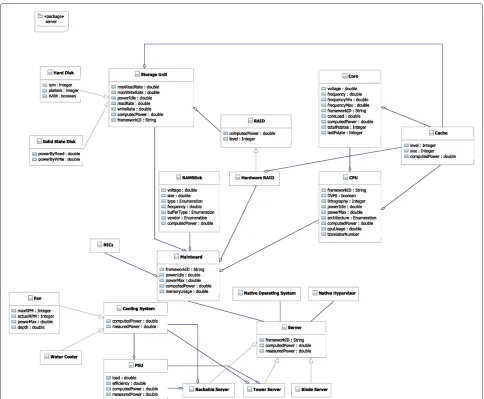
Figure 5Server UML class diagram.The figure, which is a Unified Modeling Language design, illustrates in detail the different components such as processors, mainboard, memories, hard disks that a server can be composed of.
The “RAMStick” class has several attributes relevant to power consumption estimation:voltagereflects the sup-ply voltage under which the memory module operates which is highly dependent on thetype(e.g. DDR1, DDR2, DDR3, etc.), whereassizeandfrequencyindicate respec-tively the size (in GB) and frequency (in MHz) of the mem-ory,vendor denotes the manufacturer (e.g. KINGSTON, HYNIX, etc.), bufferType shows the type of the mem-ory module in terms of buffer technology (e.g. fully buffered, buffered, registered, and unbuffered). It is worth-while to mention that values of all the above-mentioned attributes are provided by the manufacturer’s data sheet.
Several “Storage Unit”s can be attached to a “Server” either directly through its “Mainboard” or by means of a dedicated “Hardware RAID” device. Additional information regarding storage modelling is provided in
Section Storage modelling. As mentioned previously, “Tower Server”s and “Rackable Server”s are equipped with their own Power Supply Units (“PSU” class) and cooling systems (“Cooling System”) which can be either a “Water Cooler” or a “Fan”. The followings are the most relevant energy-related attributes of a “PSU”:efficiency(in percent-age) indicates the amount of loss of the power supplied to the components of the server, which is highly related to theload. Note that values of efficiency for the correspond-ing loads can be extracted from the manufacturer’s data sheet.
whose value should be kept up-to-date through the data centre’s monitoring system.
Storage modelling
In this section, we present the storage modelling both for the case of storage units attached directly to servers as well as the case of Storage Area Network (SAN) devices. A generic UML class diagram for these cases is introduced in Figure 6.
Server storage
Left part of the UML class diagram of Figure 6 illustrates the server storage modelling where the “Storage Unit” class represents the abstraction for all kinds of disk-like devices providing the physical storage for data. “Storage Unit”s can be directly connected to a “Server” through
its “Mainboard” or by means of a “Hardware RAID” controller that provides the differentlevelsof RAID sup-port to servers. We consider both traditional disks with revolving platters (“Hard Disk” class) and solid state disk (“Solid State Disk”) as possible “Storage Unit” devices. Note that attributes for “Server” and “Mainboard” classes are described in Section Server modelling.
“Storage Unit” class’ energy-related attributes are the followings: maxReadRate and maxWriteRate indicate respectively the maximum read and write rates of the disk which are computed in terms of the transferred size per second (MB/s). The values for above-mentioned attributes can be extracted from the manufacturer’s data sheet. read-RateandwriteRateindicate respectively the actual read and write rates of the disk which are expressed in terms of MB/s as mentioned previously. The values for both of
these attributes should be kept up-to-date through the data centre’s monitoring system.
Each “Hard Disk” has the following different energy-related attributes:rpmindicates the rotation per minute of the disk, platters denotes the number of platters, whereasAAMpresents whether the hard disk is equipped with Automatic Acoustic Adjustment feature. For the “Solid State Disk”,powerByReadandpowerByWritedenote respectively the power consumed by read and write oper-ations. The distinction here is due to the fact that read and write operations in solid state disks have different power consumption behaviour.
“Storage Unit”s can also be attached logically to a “Server”. Such a functionality is provided by means of “Logical Unit”s abstraction of “SAN” devices called “LUN”, whose details are covered in Section SAN storage. Each “LUN” class has the following attributes: LUNRef is used to reference the corresponding logical unit of a SAN device, whereas readRate and writeRate have the same definition as for their counterpart of “Storage Unit” class.
SAN storage
A Storage Area Network (SAN) is a dedicated device that provides network access to consolidated, block level storage. SAN architectures are alternative to storing data on disks attached to servers or storing data on Net-work Attached Storage (NAS) devices connected through general purpose networks - which are using file-based protocols.
Right part of Figure 6 illustrates the SAN devices UML class diagram. Typically, a “SAN” device consists of more than one (usually two) “PSU” and “Fan” for redundancy purposes, several fiber channel (FC) and Ethernet Net-work Interface Cards (“FiberchannelNIC” and “Ethernet-NIC” classes) and a set of “Storage Unit”s. Furthermore, “Storage Unit”s are logically consolidated through “Logical Unit”s abstraction such that a “Storage Unit” is a member of one and only one “Logical Unit”. “Server”s access a “Log-ical Unit” through a unique log“Log-ical unit number reference (“LUN” class).
Each “SAN” class has the following energy-relevant attributes: networkTrafficIn and networkTrafficOut have the same definition as their counterparts trafficIn and trafficOut of Section Network topology modelling. On the other hand,RAIDLevelof “Logical Unit” class shows the level (e.g. RAID 0, 1, 5, 10, etc.) of the RAID being used with the corresponding logical unit. As a mat-ter of fact, each logical unit can be considered as a separate RAID controller. Furthermore,stripeSizeshows the size of the RAID protocol’s stripe. numberOfRead and numberOfWrite denote respectively the number of read and write operations performed per second. All the other attributes of “Logical Unit” class have the same
definition as their counterparts of the “Storage Unit” class of Section Server storage.
Services modelling
By the term services we mean any type of software applications which directly or indirectly generate load on ICT resources of a data centre. Consequently, all software components, either at application or system level, independently from the computing style (e.g. tra-ditional, supercomputing or cloud computing) of the data centre, can be modelled as load generator whose UML class diagram is introduced in Figure 7. Note that such a model is necessary for energy optimisa-tion algorithms that seek to distribute and potentially move software application load (e.g. virtual machine) to the computing resources which consume less power and still satisfy the required Service Level Agreements (SLA).
Physical servers (“Server” class) execute the software structured and layered as depicted in Figure 7. Above the hardware level, at start-up a physical server bootstraps either a traditional operating system (“Native Operating System”) or a virtualisation hypervisor (“Native Hypervi-sor”). Some virtualisation hypervisors need to run above an operating system (“Hosted Hypervisor”).
Figure 7Services UML class diagram.The figure, which is a Unified Modeling Language design, shows the different software components (e.g. applications, operating systems, virtual machines, etc) that can run on physical servers.
“Virtual machine”s typically boot a “Hosted Operating System”, which might contain – depending on the case – specialised drivers to operate on virtualised devices.
The UML class diagram of Figure 7 describes “Operat-ing System” class as a generalisation for a traditional native or hosted operating systems (OS), and for native hyper-visors: they all share the “boot on ” relation with respect to a physical server or a virtual machine. systemRAM-BaseUsageindicates the amount of memory allocated by
An important energy-related attribute for “Software Net-work” is switchFabricType as this indicates the type of the network device the software is emulating (switch or router).
The typical software packages (“Software Application” class) can run either on a “Native Operating System” and/or on a “Hosted Operating System”: some applica-tions don’t have problems in any execution environment, while others are not able to run in virtualised mode, thus the distinction in the model. The actual power con-sumption of the “software application ” increases with the increase of number of processing resources such as NumberOfCPUs,actualCPUUsage(load imposed on the processor), actualStorageUsage (size in GB), actualD-iskIORate(MB/s), actualMemoryUsage(size in GB) and actualNetworkUsage (packets/s or MB/s) that the appli-cation is using. Note that the values of these attributes should be kept up-to-date through the data centre’s monitoring system.
Power consumption prediction models
In this section, we introduce the power consumption pre-diction models of the most relevant ICT resources of data centres such as servers, storage devices and net-working equipment (e.g. routers or switches). Note that such power consumption models are the cornerstone of energy optimisation algorithms by providing them with detailed insights regarding the power consumption of the aforementioned ICT resources in different workload deployment configurations.
Server
The power consumption of a server is broken down into two parts: idle and dynamic. The former is computed while the server is idle with no activities, whereas the lat-ter is calculated when the server is performing certain computations. As a matter of fact, it is necessary to model both aspects for different components of a server illus-trated in Figure 5, in order to have a deeper understanding on the power consumption.
Processor
It was shown in [13] that processors are the most promi-nent contributors (about 40%) to the overall power consumption of servers. Furthermore, the power con-sumption of processors can be due to either its idle state (no utilisation) or dynamic state while carrying out certain computations. With the advent of multi-core pro-cessors (e.g. dual-core, quad-core, etc.) as well as their corresponding energy-efficient mechanisms (e.g. Intel SpeedStep, AMD Cool’n’Quiet), several techniques (e.g. Dynamic Voltage and Frequency Scaling - DVFS) were introduced that save energy especially when the processor is in idle or low utilisation states.
Idle power consumption The idle power consumption of a processor can be determined by using the following well known equation [26] derived from Joule’s and Ohm’s laws:
P=I∗V, (1)
where P denotes the power (Watt), I represents the electric current (Ampere) and V indicates the voltage. Equation (1) can be adopted in order to compute the idle power consumption at core level by assuming that each core contributes equally to the overall idle power consumption of a processor:
Pi=Ii∗Vi, (2)
wherePi,IiandVidenote respectively the power, current and voltage of the corresponding corei. Furthermore, by analysing the current Ii and voltage Vi relationship, we derive the following second order polynomial (using the curve-fitting methodology) to model the current leakage:
Ii=αVi2−βVi+γ, (3)
where α = 0.114312 ((V)−1), β = 0.22835 (−1) andγ = 0.139204 (V) are the coefficients such that V anddenote respectively the voltage and resistance. It is worthwhile to note that these values are derived based on results obtained from a power meter [27] while analysing a quad-core processor with energy-efficient mechanisms (e.g. DVFS) deactivated.
With the emergence of energy saving mechanisms (e.g. Intel SpeedStep, AMD Cool’n’Quiet), the idle power con-sumption of a core (processor) decreases. This is achieved by decreasing the voltage and frequency (DVFS) of a core. In order to demonstrate such an impact, we propose the following model:
Pri=δiPi, (4)
where δi is the factor for reduction in the power con-sumption Pi of core i (see Equation (2)), whereas Pri
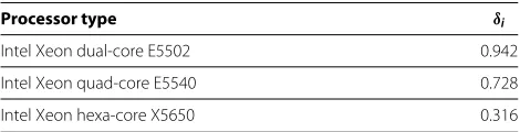
represents the reduced power consumption of core i. It is worth pointing out that δi can vary depending upon the corresponding energy saving mechanisms where each of such mechanism has its own particular features (the detailed modelling ofδiis out of the scope of this paper). To this end, in this paper we provide values of δi for multi-core Intel processors in Table 1. Certain processors, for instance, Intel dual- and quad-core processors do not possess deep C-states. Hence, the energy reduction fac-tor for processors (e.g. hexa-core) having such states is significantly different from the others.
Table 1 Values ofδifor Intel Processors
Processor type δi
Intel Xeon dual-core E5502 0.942
Intel Xeon quad-core E5540 0.728
Intel Xeon hexa-core X5650 0.316
The values of the reduction factorδifor different types of Intel processors.
PCPUidle =
n
i=1
Pri, (5)
wherePriis introduced in Equation (4).
Dynamic power consumption The power consumption of theithcore of a multi-core processor due to performing certain computations is given by:
Pi=Pmax Li
100, (6)
where Pi denotes the dynamic power consumption of the coreihaving a utilisation (load) ofLi, whereasPmax indicates the maximum power consumption due to 100% utilisation. It is worthwhile to note that Equation (6) is derived based on the well known linear utilisation-based model of [13] for single-core processors.
The maximum power consumptionPmax is computed by adopting the following well known CMOS [28] circuits power consumption equation:
Pmax=Vmax2 ∗fmax∗Ceff, (7)
whereVmaxandfmaxdenote respectively the voltage and frequency at maximum utilisation, whereasCeff [28] indi-cates the effective capacitance which includes the capaci-tanceCand switching activity factorα0→1.
Given a processor ofncores with no specific energy-saving mechanisms enabled, then its dynamic power con-sumption is given by:
PCPUdynamic =
n
i=1
Pi, (8)
wherePiis introduced in Equation (6).
In fact, there are certain factors which play a major role in reducing the overall power consumption of multi-core processors of Equation (8). Among those, the followings are two main techniques through which the power con-sumption of multi-core processors can be reduced: Energy saving mechanisms such as Intel SpeedStep and AMD Cool’n’Quiet decrease power utilisation of a core by con-trolling its clock speed and voltage dynamically. In the idle mode or when the utilisation (load) of a core (pro-cessor) is low, the clock speed is reduced to minimise its power dissipation. Resource sharing (e.g. L2-cache in case of certain Intel multi-core processors) reduces the
power consumption. We believe that this assumption is true due to the fact that sharing L2-cache with other cores minimises the cache miss ratio. As a consequence, less communication takes place with the memory (e.g. to fetch new instructions), which contributes in reducing the total power consumption of cores.
Due to these power reduction mechanisms, the power consumption of a multi-core processor is always less than the one of Equation (8). In order to cope with this over-estimation, we introduce a power reduction factor (δ) to Equation (8) in the following manner:
PCPUdynamic =δ(
n
i=1
Pi), (9)
where the detailed modelling ofδ is not covered in this paper. However, it is worthwhile to mention the following facts related to the modelling ofδ:
1. The reduction factorδchanges by modifying the
frequency of the processor.
2. The number of active (a utilisation of more than 1%) cores of the processor has an impact on the
reduction of power consumption.
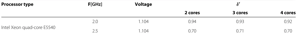
Table 2 illustrates a sample value ofδ for an Intel quad-core processor having different number of 100% loaded cores as well as clock frequencies ranging from 2.0 to 2.5 GHz. As we can notice, the higher the frequency is, the possibility of reducing power becomes more evident. Fur-thermore, more power is saved as the number of active cores increases. These are due to the fact that the pure summation of the power consumption of the cores given by Equation (8) is always greater than the total actual power consumption. As a matter of fact, this difference becomes important for increasing frequencies and num-ber of active (100% loaded) cores. Hence the reduction factorδbecomes more obvious for those cases.
Total power consumption The total power consump-tion of a multi-core processor is defined by:
PCPU=PCPUidle +PCPUdynamic, (10)
wherePCPUidleandPCPUdynamicare introduced in Equations
(5) and (8) respectively.
Memory
Table 2 Values ofδbased on Frequency and Number of 100% Loaded Cores
Processor type F[GHz] Voltage δ
2 cores 3 cores 4 cores
2.0 1.104 0.94 0.93 0.92
Intel Xeon quad-core E5540
2.5 1.104 0.70 0.71 0.70
The values of the reduction factorδfor different frequencies of Intel quad-core processor. The reduction factor also changes based on fully loaded cores.
With respect to the idle power consumption of DDR3 memory, we derive a model starting from the following well known equation [26] :
P=I∗V, (11)
wherePdenotes the power (Watt),Irepresents the elec-tric current (Ampere) andVindicates the voltage. On the other hand, it was shown in [29] that there is a linear rela-tionship between the current I and voltageV when the supplied voltage is between 0 and 2V (which is typically the case for DDR3 memory). Hence the current can be expressed in the following manner:
I=c∗V, (12)
where based on our observations, we noticed thatctakes a value of 13 × 10−5. Taking Equations (11) and (12) into account, the power consumption of a DDR3memory module for a given frequencyf (in MHz) and sizes(in GB) can be rewritten in the following way:
P(f,s)=c∗V2. (13)
Consequently, in order to reflect the impact of frequency on the idle power consumption, Equation (13) can be written as:
P(s)=f ∗c∗V2. (14)
Furthermore, in order to show the influence of size (in GB) on the idle power consumption, Equation (14) can be written as:
P=s∗f ∗c∗V2. (15)
Given a set ofnDDR3memory modules, then their idle power consumption is expressed as:
PRAMidle =
n
i=1
si∗fi∗c∗Vi2, (16)
wheresi,fiandVidenote respectively thesize(in GB), fre-quency (in MHz) and the voltage (volts) of a specific DDR3 memory modulei, whereasctakes a value of 0.00013.
Concerning the dynamic power due to accessing the memory, there is always only one active operating rank per channel regardless of the number of memory modules or module ranks in the system. As a matter of fact, such a power is always constant during access and independent
of the operation type (read or write) as well as size and is given by:
PRAMdynamic =9.5 Watt, (17)
Then based on Equations (16) and (17), the overall power consumption of a Random Access Memory is given by:
PRAM=PRAMidle+γ ∗PRAMdynamic, (18)
where γ ∈[ 0, 1] whose details are covered next. Since certain monitoring systems (including the one of our real-world testbed) can not provide information about how often the memory modules are accessed, then we adopted the following technique to derive values forγ:
1. If the processor is in idle state performing no activity, then we assume that the memory modules are also in
idle state (γ =0).
2. If the processor is carrying out certain computations (utilissation of more than 1 %), then we adopt a
probabilistic approach in modellingγ, such that the
more total memory is in use, the higher in probability that a memory access is performed:
γ = memoryUsagen i=1si
, (19)
where nandsi are defined in Equation (16) and memo-ryUsageis introduced in Section Server modelling.
Hard disk
Typically, the power consumption of a hard disk can be broken down into three major parts: startup, idle, andaccessing modes, where each such mode has differ-ent power consumption behaviour. The disk is in startup mode when all of its mechanical and electrical compo-nents are activated. On the other hand, the disk is in idle mode when no activity (read or write) is carried out, whereas it is in accessing mode while performing read or write operations.
and sleep states, the disk’s mechanical parts are signifi-cantly stopped. Then, the idle mode power consumption of the hard disk is given by:
PHDD idle=Pidle(α+0.2∗β), (20)
such thatα∈[ 0, 1] indicates the probability that the disk is in idle state,β ∈[ 0, 1] denotes the probability that the disk is in standby and sleep states (the values ofα andβ are given later such thatα+β = 1), whereasPidleis the idle state power consumption provided by the manufacturer’s data sheet. Furthermore, we observed that the startup and accessing modes’ power consumption is respectively in average 3.7 and 1.4 times more than that of the idle state power consumption. Then, the power consumption of the hard disk is given by:
PHDD=x∗1.4∗Pidle+y∗PHDD idle+z∗3.7∗Pidle, (21)
such thatx,y,z ∈[ 0, 1] denote respectively the probabil-ity that the disk is in accessing, idle and startup modes, whereasPidleis the idle state power consumption provided by the manufacturer’s data sheet.
Since certain monitoring systems (including the one of our real-world testbed) can not provide information about when each hard disk switches from startup, to idle and accessing modes, then we adopted the following two tech-niques in order to derive values forx,yand z such that x+y+z=1:
1. If the average operation size (MB/s) of reads and
writes per second is zero (readRate=writeRate
=0), then we assume that the disk is in its idle mode
(x=z=0andy=1).
2. If the average operation size (MB/s) of reads and writes per second is not zero, then we adopt a probabilistic approach in modelling the mode changes such that:
• IfreadRate>0andwriteRate>0, then
x= maxReadRate+maxWriteRatereadRate+writeRate ,
• IfwriteRate=0, thenx= maxReadRatereadRate ,
• IfreadRate=0, thenx= maxWriteRatewriteRate ,
Note that readRate, maxReadRate, writeRate and maxWriteRate are introduced in Section Storage mod-elling, whereasy = 0.9∗(1−x)andz = 0.1∗(1−x). Finally, in order to derive values ofα,β ∈[ 0, 1] for the idle mode power consumption, we adopted the following probabilistic approach:
1. If0<y≤0.3, then we setα=0.9andβ= 0.12.
2. If0.3<y≤0.6, then we setα=0.5andβ= 0.52.
3. If0.6<y≤1, then we setα=0.1andβ= 0.92.
We can notice from the above equations that the more the hard disk is in idle mode (y 1), the higher is the probability that it will remain in standby and sleep states.
Network interface card
Network interfaces, which connect a server to one or more networks, normally operate at a fixed line rate and add both physical and link layer functionalities that con-tribute to increase the total power consumption of a server. At any given time, a network interface will be either in idle mode or actively transmitting or receiving packets. IfPNICidle is the power of the idle interface andPNICdynamic
is the power when active either (or both) receiving or transmitting packets, the total energy consumption of an interface will be given by:
ENIC=PNICidleTidle+PNICdynamicTdynamic, (22)
whereTidleis the total idle time andTdynamicdenotes the total active time in an observation period T = Tidle+ Tdynamic, such that Tidle andTdynamic > 0. The average powerPNICduring periodTis:
PNIC=
(T−Tdynamic)PNICidle+PNICdynamicTdynamic
T
=PNICidle +(PNICdynamic −PNICidle)ρ (23)
whereρ = TdynamicT is the channel utilisation (also known as the normalised link’s load). Both time periods and power values would depend on the particular network technology employed.
It is interesting to note that the choice of network tech-nology could affect, to varying degrees, the utilisation of other computer system components and in particular pro-cessor (CPU). For example, in serial point-to-point (PPP) communications, the CPU is normally used to execute a significant number of communication-related opera-tions (e.g. frame checking and protocol control). These operations can easily increase the dynamic power con-sumption of the CPU. On the other hand, embedded network implementations, such as InfiniBand, can move much of the communication work to the embedded archi-tecture. To include this network-technology dependent behaviour into our model, consider parameter Li (CPU load) in Equation (6) as resulting from two components: Li=L
i+γρ, whereL
Mainboard
The aggregated power consumption of the mainboard consists that of its constituent components attached to it and is given by the following equation:
PMainboard= l
i=1
PCPU+PRAM+ m
j=1 PNIC+
n
k=1
PHDD+c,
(24)
where PCPU, PRAM, PNIC, and PHDD are given respec-tively by Equations (10), (18), (23), and (21), whereascis constant related to the mainboard’s own power consump-tion. Note that technically it is challenging to compute the power consumption of the mainboard. Hence, statistical values forccan be derived based on the server type (e.g. tower, rackable, and blade), which is reflected by means ofpowerIdleandpowerMaxattributes of the “Mainboard” class in Section Server modelling.
Fan
The power consumption of a fan changes from one Rota-tion Per Minute (RPM) to another: i.e. the higher the RPM is, the more power it consumes. Consequently, a model is derived starting from the following well known formulab for the power consumption of a fan:
P=dp∗q, (25)
wherePdenotes the power consumption (Watt),dp indi-cates the total pressure increase in the fan (Pa or N/m2), andqrepresents the air volume flow delivered by the fan (m3/s). Hence, replacingdpby FAandqby Vt in Equation (25), we obtain:
P= F A∗
V
t , (26)
whereF,A,Vandtdenote respectively the force (N), area (m2), volume (m3) and time (seconds). By a simple simpli-fication of volumeV and areaA, we obtain the following equation:
P= F∗d
t , (27)
whereFdenotes the force (N),dindicates the depth of the fan (m) andtrepresents the time (seconds). Based on our observations performed on a set of fans, we found out that Fis proportional to the square of the RPM:
F=c∗RPM2. (28)
By taking into account Equations (27) and (28), the power consumption model for the fan is given by:
PFan=
c∗RPM2∗d
3600 . (29)
whereRPMdenotes the actual rotation per minute of the fan (actualRPMin Section Server modelling) whose value
should be kept up-to-date through the monitoring system. It is worthwhile to note that for a given fan, the value of cremains constant. As a matter of fact, we compute the value ofcbased on Equation (29):
c= 3600∗Pmax RPM2
max∗d
, (30)
where Pmax andRPMmax denote respectively the maxi-mum power and rotations per minute of the fan whose values can be extracted, in addition to the depthd, from its manufacturer’s data sheet.
Power supply unit
As its name indicates, PSU supplies power to the numer-ous components of a server. In general, the power con-sumed inside the PSU itself (loss) is highly dependent on its efficiency: the higher the PSU is in efficiency, the less power it consumes. To this end, the PSU manufacturers provide the efficiency range with respect to a given PSU load. Hence, we compute the power consumption of a PSU having anefficiencyofe, in the following manner:
1. If the data centre’s monitoring system provides information at the PSU level (measuredPower of “PSU” class in Section Data centre schema), then the power consumption is given by the following equation:
PPSU =
measuredPower∗(100−e)
100 .
2. If the data centre’s monitoring system provides information only at the server level (measuredPower of “Server” class in Section Data centre schema), then
we assume that thismeasured power of the server is
evenly distributed among itsn PSUs (having similar
efficiency) providing power to the components, and compute the power consumption by the following equation:
PPSU =
(measuredPowern )∗(100−e)
100 .
3. If the data centre’s monitoring system provides no information neither at the server level nor at the PSU level, then we compute the power consumption by the following equation:
PPSU=(
PMainboard+PFan
n∗e )∗100−(
PMainboard+PFan
n ),
such thatPMainboardandPFanare introduced in
Equations (24) and (29) respectively, whereasn
denotes the number of PSUs ande their efficiency
Server power consumption
Given a server composed of a mainboard, several fans and power supply units as illustrated in Figure 5, then we compute its power consumption in the following manner:
1. If the server is of typeBlade, then its power
consumption is given by the following equation:
PBlade=PMainboard. (31)
2. If the server is of typeTower or Rackable, then its
power consumption is given by the following equation:
PTower Rackable=PMainboard+ l
i=1 PFan+
m
j=1 PPSU,
(32)
such thatPMainboard,PFanandPPSUare respectively given by Equations (24), (29), and Section Power supply unit.
SAN devices
Given a SAN device whose UML class diagram is depicted in Figure 6, then its power consumption is presented by the following equation:
PSAN=PSANidle +PSANdynamic, (33)
such thatPSANidle andPSANdynamic denote respectively the
idle (no activity) and utilisation dependent power con-sumptions. Moreover, the idle power consumption of the SAN devices is given by:
PSANidle=
n
i=1
PHDD idle+ m
j=1
PENICidle+
l
k=1
PFCNICidle+c,
(34)
wherendenotes the total number of installed hard disks whose idle power consumption is given by Equation (20), m and l indicate respectively the total number of Eth-ernet Network Interface Cards (NIC) and Fiber Channel NICs having an idle power ofPENICidleandPFCNICidlegiven
by manufacturer’s data sheet, whereas c is a constant value representing the idle power consumption due to the mainboard and its attached components other than those mentioned above. Statistical values forccan be configured bypowerIdleattribute of the SAN devices introduced in Section SAN storage. It is worthwhile to note that most of the real-life cases, such SAN devices rarely go to sleep or standby modes. As a matter of fact, we setα = 1 and β=0 for Equation (20).
On the other hand, the dynamic power consumption of a SAN device is as follows:
PSANdynamic =
r
o=1
PLU(o)+
s
p=1
PENICdynamic
+
t
q=1
PFCNICdynamic, (35)
where p and q denote respectively the total number of Ethernet and Fiber Channel NICs whose dynamic power consumption is given by Equation (23), whereaso indi-cates the total number of Logical Units of a SAN device whose dynamic power consumption is:
PLU(i)=(
NbRi NbRi+NbWi
) ri
i=1 PHDD
+( NbWi
NbRi+NbWi )
wi
j=1
PHDD, (36)
such that NbRi and NbWi denote respectively the total number of read and write operations performed per second which are represented by numberOfRead and numberOfWrite attributes of “Logical Unit” class in Section SAN storage, whereas PHDD is the power con-sumption of the corresponding hard disk introduced in Equation (21). Since it is not possible for monitoring systems of data centres to provide accurate information regarding whether the last performed operation is read or write, then we adopt a probabilistic approach in Equation (36) by using the number of read and write operations per-formed per second in order to guess which operation has more dominance. Note that such a guess is important for RAID protocols since the number of involved hard disks differ from read to write.
In order to compute the number of involved hard disks ri due to performing a RAID protocol read operation at Logical Uniti, we apply the following technique:
|Ri| = λi
NbRi
, (37)
where λi denotes the read rate (MB/s) of the Logical Unitirepresented byreadRateattribute of Section Server storage and|Ri|indicates the average read operation size (MB/read) per second. Based on Equation (37), the num-ber of involved hard disks is given by:
ri= | Ri|
stripeSize, (38)
picked up randomly since this is purely RAID level’s pro-tocol dependent. As a matter of fact, we assume that the hard disks attached to a given Logical Unitihave similar power consumption behaviour.
Network equipment
Given that the power consumption PNEQ of a network equipment will be mainly driven by the internal switch-ing state and buffer utilisation, it is sensible to assume that its overall power consumption will be linked to its total packet switching throughput (λ):
PNEQ=γ+ (λ), (39)
where γ represents the power consumed by the equip-ment without workload and (.) a function that deter-mines the level of power used by a given packet switching throughput. The exact form of function (.)will be deter-mined by the implementation technology. In practical terms, the contribution of (.) to the total power con-sumption of a regular (embedded) network equipment is expected to be small. However, it is also expected that this trend will change in the future as “greener” implementa-tions are introduced.
Evaluation and results
Testbed environment and configuration
The testbedc under investigation provides a computa-tional environment implementing cloud computing for Infrastructure as a Service (IaaS) platform. It is the most basic cloud service typology, where virtual infrastructure resources (e.g. CPU, memory, storage devices) are pro-vided to users on dynamic and scalable basis. It is worth-while to note that the testbed is based upon a Lab-grade infrastructure fully resembling (in a smaller scale) both the configuration and functional capabilities of actual production-grade IaaS implementations, being private or public.
Hardware configuration
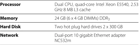
The hardware equipment consist of two racks each host-ing an HP Blade System C3000 [30] enclosure where equivalent ISS (Industry Standard Server) blade servers are mounted inside. In addition to the four free slots, each enclosure bears 4 blade servers (a total of 8 in the testbed) belonging toHP ProLiant BL460c G6[31] series which are half-height blades, configured as in Table 3.
Inside each enclosure, the servers are interconnected through anHP Virtual ConnectEthernet Module. The two racks, in turn, are interconnected through an external Eth-ernet switch. Power supply is bundled with the enclosure, through 6 high efficiency (90%) 1200WHP Common-Slot Power Supply Units. Cooling is provided by 6HP Active Cool 100fan units, also directly installed in the enclosures.
Table 3 Servers’ Hardware Configuration
Processor Dual CPU, quad-core Intel Xeon E5540, 2.53 GHz 8 MB L3 cache
Memory 24 GB (6 x 4 GB DIMMs) DDR3
Hard Disk Two hot plug hard drives 2 x 300 GB Network Dual-port 10 gigabit Ethernet adapter
NC532m
The hardware characteristics of the servers for the corresponding testbed regarding.
Finally, energy measurement is performed by an HP hardware component namediLO(Integrated Lights-Out), accessible through theInsight Controlsoftware suite.iLO offers the ability to read real-time electrical power con-sumption down to single server level.
Software configuration
The testbed’s architecture consists of the following five software components:
1. The Cloud Controller (CC), 2. The Node Controller (NC), 3. Energy-aware plug-in,
4. The Power and Monitoring Collector (PMC), 5. The client (end user) system.
The Cloud Controller (CC) is the component hosting the core cloud management functions, i.e. it’s the application server (Front End) where the cloud web services actu-ally reside. These services are triggered by any end user request, asking to activate or deactivate a set of computa-tional resources, identifiable as virtual machines. Further-more, the CC software is deployed onto a physical server, as typically done to duly keep under control the response time to client requests. This software runs on a Red Hat Enterprise Linux (RHEL) 5.5 operating system instance.
a XEN hypervisor, and typically host Linux images (e.g. Ubuntu, Suse, Red Hat, etc.).
The energy-aware plug-in (described briefly in Section Contributions and results) resides altogether on a dedicated virtual machine, running on the VMware ESX 4.0 hypervisor. The Power and Monitoring Collec-tor (PMC) is implemented by a customised version of collectd. Collectd is an open source Linux daemon able to collect, transfer and store performance data of com-puters and network equipment. For our testbed, specific collectdagents have been developed and implemented, to interface withiLOand acquire power measurement data. Like the Cloud Controller, even the PMC is deployed on a physical server.
Finally, the client systems are emulated by a custom soft-ware tool, generating sequence of requests that faithfully replay the interaction among a group of observed users from a real life context and the cloud IaaS infrastruc-ture. The client load simulation is deployed inside virtual machines running an Ubuntu image, whose execution is scheduled and coordinated by a custom component run-ning on the same VMware node where the energy-aware plug-in is also deployed.
Testing methodology
A cloud computing IaaS load is by definition fairly unpre-dictable in the sense that its instantaneous computational load fluctuates arbitrarily between zero and maximum available capacity of the physical resources. This unpre-dictability in load is due to accommodating requests com-ing from a group of users, without becom-ing constrained into a static planning of the infrastructural capacity. To this regard, finding a suitable testing methodology is challeng-ing due to the lack of upfront clue on the actual usage pattern of the environment.
To overcome this methodological problem, the activities (over a period of 6 months) of a real cloud computing IaaS environment were traced and the system parameters of each active physical and virtual resource were monitored.
Then from these observations, a collection of repeating test sequences and usage patterns were extracted that altogether provides an exhaustive representation of sys-tem states worth experimenting our optimisation algo-rithms and measuring their actual results. To this end, a custom workload simulator was designed and devel-oped. This tool can generate a sequence of actions and direct them to the Cloud Controller (CC), creating the required workload snapshots in order to enact energy-aware optimisation algorithms and measure the achieved results with the best significance.
The testbed is equipped with a data logger component, storing all the details of the energy-aware plug-in activi-ties, along with the measured energy and the correspond-ing timestamps. After the end of the proof of concept, the log files were extracted from the system, and care-fully analysed to take out of them a perceptible track of the actual user activities performed and logged. As a final outcome of this hindsight, we obtained crisp and content-relevant activity profiles of 7 different usage patterns. The chosen profiles span a sufficient timeframe and content to get a significant variance of activity profiles, and a suffi-cient amount of dynamical context changes (new activities and tasks, high load versus night timeframes). These pro-files serve as the basis for designing and implementing the workload patterns enacted by the simulator tool whose details are covered next.
Workload generation
Based on the observations of the real case user activity profiles as explained in previous section, a basic set of activity types is identified typically replicable on a weekly basis. The analysis elucidated the existence of overall three basic activity aggregation types, detectable in different profiles per user and per virtual machine:
1. Steady tasks: spawn a virtual machine, and keep it running for a medium-long period of time, with a basically constant level of resource usage (e.g. CPU,
Figure 9Idle power consumption of blade servers.The figure shows the idle power consumption of blade servers obtained from a power monitoring tool (iLo) and developed power consumption models (PCM).
memory, storage device); typical cases were complex software application development tasks.
2. Spiky tasks: spawn a virtual machine, intensively use it for a short term period (e.g. a quick debug on an application), then suddenly release it to the IaaS environment.
3. Rippling tasks: spawn a virtual machine, and keep it running for a medium-long period of time, with a fairly variant pattern of resource usage; this typology can be associated, for instance, to data
management/reporting activities, or to some particular tasks ran in collaboration.
After identifying the above-mentioned three basic activ-ity types, the next step was to configure the workload sim-ulation tool in order to generate a realistic sequence of sys-tem actions (create and de-instantiate virtual machines) able to replicate as faithful as possible these recovered patterns.
A snapshot of a workload profile is shown in Figure 8. It is worthwhile to mention the fact that time schedules have been squeezed into a 7:1 or 7:2 compression factor. As a matter of fact, all the tests of one week long are per-formed in a single day or 2 days time slot, ensuring the full execution of the test plan. Before going full speed with the test campaign, we ran a single-spot, full week test on a selected sample profile, followed by the time squeezed test on the same profile, to make sure that the time compres-sion didn’t bring up any bias or alteration to the observed system behaviour.
Numerical results
Power consumption predictions
Before performing our tests related to the energy opti-misation, it was necessary to validate the accuracy of the power consumption prediction models of Section Power
consumption prediction models. To this end, we carried out observations both for the idle and dynamic power consumptions of the blade servers whose hardware con-figuration is presented in Table 3.
Idle power consumption predictions Figure 9 illus-trates the power consumption of the blade servers both obtained from our power monitoring tool iLO and our power consumption prediction models (PCM). We can notice that both have identical power consumption which is due to the fact that we were able to config-ure the mainboard power consumption (seepowerIdlein Section Server modelling) appropriately. In Table 4, we present the idle power consumption breakdown on the component-basis.
Dynamic power consumption predictions In order to better understand the power consumption behaviour of our blade servers under different load patterns, we per-formed tests (1) by explicitly fixing the frequency of the processor to its maximum and (2) by letting the operating system to configure it automatically (e.g. on-demand gov-ernor) based on certain OS-related mechanisms ensuring
Table 4 Idle Power Consumption Prediction Breakdown
Component Consumption(Watt)
Processors 33 Watt
Memories 14 Watt
Hard Disks 3 Watt
Mainboard 70 Watt
Total 120 Watt
Figure 10Power consumption of blade servers with dynamic setting.The figure demonstrates the power consumption of blade servers obtained from a power monitoring tool (iLo) and developed power consumption models (PCM), by increasing the load of the processors by increments of 20%. The frequency of the processors are configured dynamically by means of the operating system in order to achieve the required performance.
performance and energy efficiency (e.g. Intel SpeedStep). To identify the trend of the power consumption for a server, we adopted the lookbusyd software tool, which allows to generate synthetic workload on a server in a tractable way, based on a wide set of parameters (e.g. CPU usage, memory usage, IO operations, etc.). The method-ology followed for testing a server was the following:
1. Set the server’s power management policy (e.g. performance, on-demand, etc.).
2. Measure power consumption fromiLO with CPU in
idle state.
3. While the CPU utilisation is less than 100%:
(a) Increment by 20% the workload on the server.
(b) Wait for a 10-minute period, to let the server and the power metering system to reach a stable situation.
(c) Measure the power consumption.
Such a measurement was repeated while simulating also memory usage with thelookbusytool, to assess the impact of memory usage on the power consumption.
Figure 10 illustrates the power consumption of the blade servers with dynamic setting (e.g. on-demand governor) both obtained from the power monitoring tooliLOand our power consumption prediction models (PCM). The horizontal axis represents the load percentage (utilisation) of all the cores: i.e. for a quad-core processor, a load of 20% reflects the fact that all the four cores are 20% loaded.