Manuscript Title & Authors

e-ISSN: 2278-7461, p-ISSN: 2319-6491

Volume 7, Issue 5 [May 2018] PP: 04-09

Selection of Linear Mixed Models to Estimate the Amount of Zinc

(Kg/Ha) On Jalo Bean

Michele Barbosa

, Leila Maria Ferreira

, Laís Mesquita Silva

, Augusto

Ramalho De Moraes

1

PhD student in Agricultural Statistics and Experimentation, Federal University of Lavras, Brazil; Theater of the Federal University of Alfenas, Campus Varginha, Brasil,

2_{PhD student in Agricultural Statistics and Experimentation, Federal University of Lavras, Brazil,} 3_{PhD student in Agricultural Statistics and Experimentation, Federal University of Lavras, Brazil,}

4_{Teacher of the Department of Agricultural, Federal University of Lavras, Brazil} Corresponding Author: Michele Barbosa

Abstract

:

Keywords:

--- --- Date of Submission: 05-05-2018 Date of acceptance: 21-05-2018 ---

---I INTRODUCTION

Cultivated by small and large producers, in diversified production systems and in all Brazilian regions, common bean is of great economic and social importance. Depending on the cultivar and the ambient temperature, it can present cycles varying from 65 to 100 days, which makes it an appropriate crop to compose, from intensive irrigated intensive farming systems to those with low technological use, mainly subsistence. The variations observed in consumer preferences, guide the technological research and direct the production and commercialization of the product, since the Brazilian regions define well the preference of common bean grain consumed.Some characteristics such as the color, size and brightness of the grain can determine its consumption, while the color of the halo may also influence the commercialization. The smaller and opaque grains more accepted than the larger ones and they have a brightness. The preference of the consumer guides the selection and obtaining of new cultivars, requiring not only good agronomic characteristics but also commercial value in retail (EMBRAPA, 2016).

Mixed models mainly used to describe the relationships between a response variable and the covariates in data that grouped according to one or more classification factors. Examples of pooled data included: longitudinal data, repeated measure data, multilevel data and block design. By associating common random effects with observations that share the same level of a classification factor, mixed models represent the covariance structure induced by clustering of data (PINHEIRO and BATES, 2000).

II MATERIALANDMETHODS

In the present study Zinc data were used in a randomized complete block design with three replicated. The treatments arranged in the parcel scheme subdivided, being the plots represented by the two environments. In the sub-plot, factorial 5x7, involving five planting densities (75, 145, 215, 285 and 355 thousands plants ha-1) and seven plant ages (13, 23, 33, 43, 53, 63 and 73 DAE, in the environment 2).

The mixed linear models allow the use of various covariance structures in the modeling process, which were first treated by Laird and Ware (1982), Jennrich and Schluchter (1986) and Diggle et al. 2002, among others.

The mixed linear model expressed as follows:

yi=Xiβ+Zibi+εi,

with i = 1, ..., c where yi represents a vector (ni × 1) of responses of the ith experimental unit or individual, Xi is

effects with zero mean and covariance matrix D and εi is a vector (ni× 1) of random errors with mean zero and covariance matrix Ri , defined positive and assuming that bi e εi has a normal distribution.

A possible model for describing the Jalo bean data is the mixed linear model that allows the efficient use of computational algorithms in which we have the yjkl response for the ith batch measured at time tij is demonstrated by the equation:

𝑦𝑖𝑗𝑘𝑙 = 𝛽0+ 𝑏0 + 𝛽1𝐵𝑙𝑜𝑐𝑘𝑖 + 𝛽2𝐷𝑒𝑛𝑠𝑖𝑡𝑦𝑗+ 𝛽3𝐸𝑛𝑣𝑖𝑟𝑜𝑛𝑚𝑒𝑛𝑡𝑘+ 𝛽4+ 𝑏4𝑙 𝑇𝑖𝑚𝑒𝑙+ 𝛽5𝑇𝑖𝑚𝑒𝑙2

+ 𝜀𝑖𝑗𝑘𝑙

(1)

We have that i = 1 , ..., 3, j = 1, ..., 5, k = 1, 2, l = 1, ..., 5. The parameters β0 to β5 represent the fixed effects

associated with the intercept, the covariates and the quadratic terms of the model. The terms b0i and b4l represent

random effects associated with the specific intercept and day-square effect for each sample i of the Jalo bean. We assume bi normal multivariate:

𝒃𝒊=

𝑏0𝑖

𝑏1𝑖

~𝑁(𝟎, 𝐃)

The term εij represents the residue associated with the observation until time tij.

𝜺𝑖 =

𝜀𝑖1

𝜀𝑖2

⋮

𝜀𝑖𝑛𝑖

~𝑁(𝟎, 𝑹𝑖)

The models obtained were adjusted by maximum likelihood andmaximum restricted likelihood, using the lme () function of R software (Pinheiro and Bates, 2000).

III RESULTSANDDISCUSSION

In order to evaluate the statistical data for zinc accumulation (Kg /ha) in the Total variable that includes (stem, leaf, leaf-stem (hf), leaf-pod (Flv), stem-leaf-pod (hfv), bean) Jalo, (Table 1)

Table 1.Mean values and standard deviation of Zinc (Kg /ha) in the Total variable.

Density Enviroment

75 145 215 285 355 pc pd

Average 27,01 33,43 37,26 42,00 58,24 36,49 42,69

Standard Deviation 26,12 23,19 26,40 34,14 46,90 36,47 30,93

Time

13 23 33 43 53 63 73

Average 6,53 15,07 24,27 44,39 58,30 62,21 66,36

Standard Deviation 3,92 8,18 12,50 31,68 25,42 40,07 33,55

A preliminary descriptive analysis of the data set may suggest models for fixed and random effects. By checking the Density variable, the highest mean registered at Density 355 and the lowest average at Density 75. For the standard deviation, the highest registered at Density 355 and lowest at Density 145.For the Environment variable, the highest mean was verified in the Environment pd and the highest standard deviation for the pc environment.

Regarding the variable Time, the highest mean registered in Time 73 and the lowest mean in Time 13. For the standard deviation, the largest deviation registered in Time 63 and the shortest deviation in Time 13.

Figure 1: Zinc accumulation (kg/ ha) in the total bean cultivar in conventional sowing (PC) and no-till (pd) over time in days (13, 23, 33, 43, 53, 63 and 73) of the plant.

The individual profiles in Figure 1 presented a specific behavior, the variability of Zn accumulation (kg/ha) being present from one unit to another with respect to the intercept, which suggests the inclusion of a random effect to this parameter.

Figure 2:Individual Zinc response profiles (kg/ha) in the total bean cultivar in conventional planting environment (pc) and no-till environment (pd) over time in plant days.

Evaluating the individual profiles of responses Figure 2 shows a trend of cubic growth in Zinc measurements over time for the five planting densities. Therefore, the third-degree polynomial is a previous candidate to represent mean growth curves.

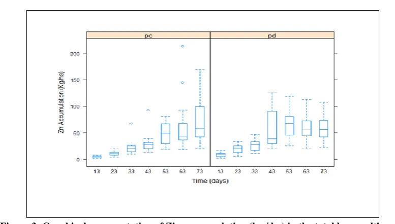
Figure 3: Graphical representation of Zinc accumulation (kg / ha) in the total bean cultivar in conventional sowing (cp) and no-tillage (pd), showing the upper and lower limits of amplitude of variation, first and third quartile and mean value of Kg / ha of Zinc in the total of the plant during the

days.

Analyzing figure 3, we can observe the presence of outliers only in the conventional plantation and at times 33, 43 and 63. In no-till, the greatest amplitude corresponds to time 43 and in conventional planting time 73. The largest median in conventional planting registered in time 73 and in no-tillage 53.

(a) (b)

(c)

Figure 4: Diagnostics of M5 model residues.

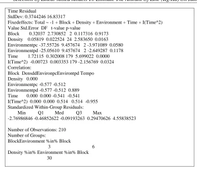
The adjustment was initiated by proposing the model M1 based on equation (1), which allows each experimental unit to have an adjusted curve, with a time and intercept angular coefficient that vary at random. The estimates of the parameters of model M1 were obtained using the function summary () of software R and the results are presented in the table below.

Linear mixed-effects model fit by REML Data: d

AIC BIC logLik 1867.141 1900.322 -923.5706 Randomeffects:

Time Residual

StdDev: 0.3744246 16.83317

Fixedeffects: Total ~ -1 + Block + Density + Environment + Time + I(Time^2) Value Std.Error DF t-value p-value

Block 0.32037 2.730852 2 0.117316 0.9173 Density 0.05819 0.022524 24 2.583650 0.0163 Environmentpc -37.55726 9.457674 2 -3.971089 0.0580 Environmentpd -25.05610 9.457674 2 -2.649287 0.1178 Time 1.72115 0.302008 179 5.699022 0.0000 I(Time^2) -0.00723 0.003353 179 -2.156769 0.0324 Correlation:

Block DensddEnvironpcEnvirontpd Tempo Density 0.000

Environmentpc -0.577 -0.512 Environmentpd -0.577 -0.512 0.889 Time 0.000 0.000 -0.541 -0.541 I(Time^2) 0.000 0.000 0.514 0.514 -0.955 Standardized Within-Group Residuals:

Min Q1 Med Q3 Max

-2.76986846 -0.46852622 -0.09193263 0.29470626 4.55838523

Number of Observations: 210 Number of Groups:

BlockEnvironment %in% Block

3 6 Density %in% Environment %in% Block 30

The Block coefficient was not significant, indicating the proposal of model M2, which does not include Block effect.

The models adjusted for the data of the quantity variable of Zinc (kg/ha), are in Table 2.

Table 2.M1 and M2 model adjustment statistics.

Model FixedEffect RandomEffe ct

gl AIC BIC p-value

M1 Intercept, Block, Density, Environment, Time and Time2

Intercept Time

10 1867,14 1900,32

M2 Intercept,Density, Environment, Time e Time2

Intercept Time

9 1868,99 1898,91 0,0495

Block maintenance tested by comparing the M1 and M2 models. The test in the comparison of M1 and M2 models was not significant (p-value = 0.0495). Opting for the M2 model as the most parsimonious model.

Adjustment of intra-individual covariance matrix structures (Ri)

When the fixed effects and random effects were chosen (model M2), the structures CS (model M3), AR (1) (model M4) and ARH (1) (model M5) were tested for the covariance matrix Ri . Table 2 shows the values of the AIC and BIC criteria, the value -2 logs for each structure.

Table 3. Adjustment statistics of models M3 to M5.

Model Ri df AIC BIC p-value

M3 CS 10 1864,23 1897,46

M4 AR(1) 10 1869,28 1902,51

M5 ARH(1) 16 1687,23 1740,40 <0,0001

Based on the results of the likelihood ratio tests and the AIC and BIC criteria presented in Table 3, the covariance structure chosen was ARH (1), being the M5 model.

The verification of the assumptions of the M5 model carried out through the graphical analysis of the residuals that allows us to state if the model presented a good fit.

Figure 4(a) shows random distribution of the around the zero value.

The histogram in Figure 4(b) and q-qplot presented in Figure 4(c) indicate that the assumption of normality for intra-individual errors is plausible. However, the presence of some outliers may justify further investigation.

IV CONCLUSION

The proposed approach was efficient in indicating the appropriate linear mixed model for the Jalo bean data set.

ACKNOWLEDGEMENTS

The authors would like to thank the financial support and scholarships granted by FAPEMIG, CAPES and CNPq.

REFERENCES

[1]. BARBOSA, Michele. An approach to data analysis with repeated using models linear mixed. 2009. Dissertation (Masters in Statistics and Agronomic Experimentation) - School of AgricultureLuiz de Queiroz, University of São Paulo, Piracicaba, 2009 [2]. DIGGLE, P .; HEAGERTY, P .; LIANG, KY; ZEGER, S. Analysis of Longitudinal Data , second edn, Oxford University Press Inc,

Clarendon. 2002.

[3]. EMBRAPA. Cultivation of common bean . Available at:

<https://sistemasdeproducao.cnptia.embrapa.br/FontesHTML/Feijao/CultivodoFeijoeiro/>. Access 17 mar. 2016.

[4]. JENNRICH, RI; SCHLUCHTER, MD Unbalanced repeated measures models with covariance matrices . Biometrics, v. 42, p. 805-20, 1986.

[5]. LAIRD, NM; WARE, JH Random effects models for longitudinal data . Biometrics, Washington, v. 38, p. 963-974, 1982. [6]. PINHEIRO, JC and BATES, DM Mixed-effects models in S and S-PLUS . New York: Springer-Verlag, 528p. 2000.