Advanced Routing Techniques for Large - Scale 2D/3D
Sensor Networks using Segmentation
1 Aparna K Menon, 2 Dr.Gnana Sheela K
1
Dept. Electronics and Communication, Toc H Institute of Science and Technology Ernakulam, India
2
Dept. Electronics and Communication, Toc H Institute of Science and Technology Ernakulam, India
Abstract - A sensor network generally consists of large number of sensor nodes which are deployed either inside the phenomenon or very close to it. Large scale 2D/3D sensor networks generally have irregular and complex topological structures. The traditional algorithms that are in use currently works well in convex geometry rather than in concave regions. Generally the existing segmentation algorithms are based on concave node detection that results in sensitivity of performance to boundary noise. In this work, the complex network is segmented into simple convex regions using connectivity based segmentation in large scale 2D/3D networks – CONSEL algorithm. The CONSEL is a scalable and distributed algorithm that is designed based on Morse function and convex components in Reeb graph of a network. The algorithm makes use of only connectivity information for segmentation. Firstly the boundary nodes in the network flood the region to construct the reeb graph. Then the mutex pairs are computed by the ordinary nodes in the region and coarse segmentation is done locally. The neighboring regions that are not mutex pairs are then merged together. It has both 2D and 3D segmentation capability. The traditional algorithm like greedy routing or geographic routing is thus adapted into a complex large scale 2D/3D environment.
Keywords - CONSEL, Routing, Morse function, Reeb graph, Mutex pairs, Concave nodes, Convex nodes.
1. Introduction
Wireless sensor networks have witnessed widespread usage in emerging applications where nodes are typically deployed in 3-D settings, such as safety monitoring of coal mine tunnels and fire detection in the corridors of buildings. A cardinal prerequisite for efficient design of a sensor network is to understand the geometry of the
environment where sensor nodes are deployed. Large scale 2D/3D sensor networks generally have irregular and complex topological structures possibly containing obstacles/holes. The traditional algorithms like geographic routing works well in convex, i.e. regular geometry rather than in concave regions. Irregular network shapes may lead to inaccurate localization results, as many existing localization algorithms assume straight-line shortest paths between nodes. This does not hold when the network topology is highly irregular, resulting in an over-estimated shortest path length and thus inaccurate localization results.
properties of the network require additional computational complexity, and many problems cannot be solved by extensions or generalizations of 2D methods. Numerous methods [14]–[17] have been proposed to improve the traditional algorithms' performance by adapting them to irregular and complex sensor field. These efforts are mostly application-specific, increasing the design complexity significantly. To tame the challenges brought by irregular shapes, convex network partitioning, also known as segmentation/convex partition was employed. In this paper, an algorithm known as CONSEL, CONnectivity-based SEgmentation in Large-scale 2D/3D sensor networks is used for partitioning the network into subregions. In CONSEL, several boundary nodes first flood the network to construct the Reeb graphs. The ordinary nodes in the network then compute mutex pairs locally, generating a coarse segmentation layout. The neighbor regions that are not mutex pair are then merged togather. Finally, by ignoring mutex pairs that lead to small concavities, we provide a configurable bound for the subnetworks’ deviation from convexity. We thus consider shape segmentation to divide a network into convex regions or subnetworks, so that traditional algorithms designed for a simple geometric region can be applied with good performance. By doing so, without heavily modifying particular algorithms, traditional algorithms are able to perform well in each convex region.
2. Background Information
In this work we resort to segmentation from a Morse function [3] perspective, bridging the convex regions and the Reeb graph of a network. CONSEL is much reliable as compared with the previous solutions. Few of its basic features are: (1) it works for both 2D and 3D sensor networks; (2) it only relies on network connectivity information; (3) it provides a bound of convexity deviation. CONSEL is distributed as no centralized operation is required, and is scalable as both its time complexity and its message complexity are linearly proportional to the network size. Extensive simulations show that CONSEL works well in the presence of holes and shape variation, always yielding appropriate segmentation results.
2.1 Concave and Convex Boundary Nodes
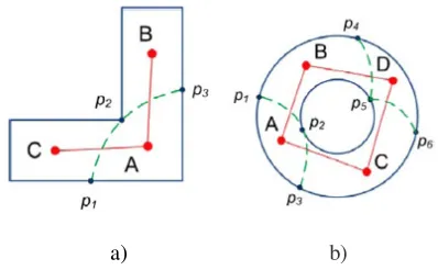
The concave nodes are nodes that are located around the concave boundaries in a network, where the boundary has an inner angle greater than π. Other nodes at regular boundaries are called convex nodes. In theory, a convex
region is a part where the line segment between every pair of its inner points lies entirely within the region.
Fig 1 Concave boundary nodes
2.2 Morse Functions and Reeb Graph
Morse Functions: For a manifold M, a Morse function [3] is a mapping f : M → R,where R is the set of real numbers, which can be considered to be a projection from higher dimensions to one dimensional manifold. That is, the outputs of a Morse function are real numbers. In this paper, the Morse function f is constructed as follows (see Fig. 1): given an origin node o, for each sensor node p in the sensor field, f(p) is referred to as the hop distance between the node p and the node o. In Fig. 2, all the nodes on the same arc have an equal value of f(·). We refer to f−1(r0) as the set of nodes whose Morse function
values are r0.
a) b)
Fig 2 Reeb graphs (red nodes and lines) of two network topologies.
nodes in Cir are r hops away from the origin node. The set of such above-mentioned neighbours is called Cir 's children set, denoted by h(Cir ). As a result, the L-components expand as the level number grows. There are three basic types of events during the transition from one L-component to its children set:
1) Extend event h(Cir ) is a maximal L-component in the (r+1)th level.
2) Split event h(Cir ). contains two or more L-components in the (r+1)th level.
3) Merge event h(Cir ). is a subset of an L-component in the (r+1)th level, which means that multiple L-components in the rth level share the same connected children set.
A series of extend events may take place in succession [say the L-components from level 1 to level 5 in Fig. 2(a)], and the involved L-components will form a connected, multilevel component of the network, called a Reeb component. A vertex in the final Reeb graph, or a Reeb vertex, represents a maximal Reeb component, and an edge in the Reeb graph, or a Reeb edge, reflects the split or merge events. Generally, a split event happens when a concave node emerges during the expanding process of L-components.
2.3 Mutex Pairs
Given a network and a Morse function, two nodes P1 and P2 are called a mutex pair, denoted by P1 ~ P2, if there exists no Morse path between them.
Given a network and a Morse function, a Morse path between two nodes P1 and P2 and is a path on which all nodes have the same Morse function value.
3. Routing Employing CONSEL Algorithm
In the implementation of CONSEL algorithm, the first and foremost step is the computation of Morse function. For this I nodes are randomly chosen along the outer boundary of the network. An arbitrary node p floods the network to find the farthest node o1 to p . Thereafter, o1 floods the network to find o2 farthest to itself. Then, o3 is the node that has the maximum sum of the square roots of the hop counts from the nodes o1 and o2.This process continues until nodes are obtained on the outer boundary. Next, each of the nodes on the boundary floods the network. First, after a flooded message from oi reaches a node p, p records the parent from which it receives the message, as well as the hop count to the node oi . By
doing so, the node has the knowledge of the Morse function value corresponding to fi(p), 1 ≤ i ≤ I. The flooding allows us to construct the Reeb graph in a distributed way.
In the next step based on the morse function computed, reeb graphs are constructed. The key to constructing a Reeb graph is to identify the Reeb components and select a Reeb landmark node for each of them, representing a Reeb vertex. Here a set of randomly selected nodes qk (1 ≤ k ≤ K) on f−1i (r) perform floodings, whose messages
contain the information of node ID, ID(qk) and hop count r. Each node on f−1i (r) will claim it is a landmark with a
given probability and broadcast to its neighbours. This kind of flooded messages is only sent to nodes exactly on f−1i (r). That is, when a node p receives the flooded
message, it compares the hop count value r with its own Morse function value fi(p). If the values are not equal, the message is discarded; otherwise, the node compares ID(qk) with the landmark ID LIDi(p) it previously received. When ID(qk) < LIDi(p) the node p will set its landmark ID to be qk (i.e., LIDi(p) ← ID(qk)) and then forwards the message to its neighbours except the node from which p receives the message. By doing so, only one landmark with the smallest ID can dominate in each connected component. We call this node a dominating landmark node. That is, all nodes in each connected component have the same landmark ID LIDi(p).
If we assume there exist two connected components for f−1i(r), corresponding to two dominating landmark nodes
q1 and q2. Under this assumption, for the nodes on f−1i (r
+ 1), several landmark nodes are found as well but few dominating landmark nodes remain. We consider three cases below.
In the first case, we find two dominating landmark nodes p3 and p4 in f−1i (r + 1). Then the edge nodes, that have
the different landmark ID with one of its neighbours, will notify the dominating landmark nodes p1 and p3 of the simplified local topology graph as shown in Fig. 3(a). In this case, a change of the number of connected components does not happen. Therefore, p3 will broadcast a message to all nodes which have LID(·) = ID(p3) on f−1i
(r + 1) so that these nodes change their landmark ID, LID(·) ← ID(p1). In such a way the simplified topology
becomes Fig. 3(d) where p2 and p4 become non-dominating landmark nodes.
In the second case, there are two kinds of nodes on f−1i (r
its neighbours has the landmark ID ID(p3). This case is shown in Fig. 3(b). In this case, a change of the number of connected component takes place. Intuitively new vertices (for simplicity, qk is considered as the vertex) should be added to the Reeb graph where one vertex represents one region. The newly generated vertices are introduced and two edges are generated on the Reeb graph.
Fig 3 Simplified local topology graph
In the last case, shown in Fig. 3(c), is similar to the second case. In this case, there is a change of the number of connected component as well. At least two dominating landmark nodes are connected to q2. The simplified topology becomes Fig. 3(e) and q3 becomes a non-dominating landmark nodes. Also, two vertices and two edges are added to the Reeb graph.
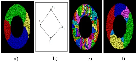
Finally all dominating landmark nodes send their local simplified topology back to the origin oi. After this phase, the origin oi has the full picture of Reeb graph based on the Morse function fi. Fig. 4(a) and Fig. 4(b) show the result of the Reeb graph after the flooding for a Morse function. In Fig. 4(a), the nodes marked with the same colour are in the same region, corresponding to one vertex in Reeb graph.
The Reeb graph is determined by the changes in the number of connected components of f −1i(r) , two distinct
connected components determined by function value range [r1, r2] is a mutex pair. All nodes in the same connected component on f −1i ([r1, r2]) should have been labelled the same landmark ID. For simplicity, these nodes record their landmark ID as ID(qk) and the dominating landmark q2 records its mutex pair dominating landmark ID ID(q3). Since I origin nodes are used, each node p records I landmark IDs accordingly. In coarse segmentation is that all nodes with the same I landmark IDs should be in one subregion. If we consider, I = 8, as an example, in which 32 dominating landmark nodes are obtained. Here each node p maintains 8 landmark IDs LID1(p), LID2(p), · · · , LID8(p) (corresponding to o1, o2, · · · , o8). Let the dominating landmark nodes be q1, q2, · · · q32.
Each of them performs flooding with its ID as subregion ID, denoted by SID(qk) (SID(qk) = ID(qk)), as well as its 8 landmark IDs LID1(qk), LID2(qk), · · · , LID8(qk). Here qk is called a representative node in a subregion if and only if ID(qk) = SID(qk). When a sensor node p receives a flooded message, it compares the landmark IDs with its own LID1(p), LID2(p), · · · , LID8(p). When they are equal, p simply discards the flooded message. If p has the same landmark IDs with the message, but it has already had one subregion ID (SID(p)) and SID(p) < ID(qk), p still discards the flooded message. Otherwise, it will update its subregion ID (SID(p) ← ID(qk)) and then forwards the flooded message to all the neighbour nodes except the message’s transmitter.
Every node has one subregion ID (SID()) and within each subregion, one node is selected to represent this subregion. The representative node SID() maintains the information of I landmark IDs in this subregion as well as I Reeb graphs to identify the mutex pair later. All subregions are the result of the coarse segmentation of the sensor network.
The next important step in the CONSEL algorithm is the merging of subregions. As we know, each representative node in the subregion maintains a landmark ID list. The representative node, say q1, sends a message, containing this landmark list LID1(q1), · · · , LIDI (q1), to another representative node, say q2, in its neighbouring subregion. If q2 does not find any mutex pair in the two landmark list, it replies a positive message to q1 to allow the merging of SID(q1) and SID(q2). The merging process is quite simple: q2 will broadcast a message to ask all nodes in its own subregion to update their subregion IDs, that is, SID() ← ID(q1). In addition, q1 will update its landmark list to include q2’s landmark list. This process will continue until no more neighbouring subregions can be merged. The result of this step is shown in Fig. 4(d) where 8 regions are finally generated.
a) b) c) d)
After the segmentation is done using CONSEL algorithm, a traditional algorithm like geographic routing is carried out within each region. After the segmentation, each node obtains a unique regional ID and knows the ID of its Reeb component landmark node, or its Reeb landmark. At the same time, the Reeb component landmark nodes can help with Inter-region routing. To that end, each Reeb landmark floods the global network to establish a shortest path tree, allowing every other node in the network to reach it via shortest path. The segmentation-assisted geographic routing is simple. When a packet is requested to route from a source node s to a destination node t, s is first greedily routed to s's Reeb landmark using the virtual coordinates. Then, the packet is routed to t's Reeb landmark via shortest path. Finally, the packet is routed to t, again using greedy forwarding based on the virtual coordinates.
4. Simulation Results
Network simulator (NS2.34) is the simulation tool used to simulate the wireless network scenario. In this work we create a large scale sensor network and have done simulations to employ geographic routing assisted CONSEL algorithm to route data from source node to destination node in the network. The same network was subjected to geographic routing to route data from source to destination nodes. Various performance metrics like packet delivery ratio, signal-to-noise ratio and energy consumption of the nodes are compared and plotted using Xgraph. The various simulation parameters used are summarized in the table 1.
A network of 371 nodes has been considered for simulations. In the large scale topology created, routing with the help of segmentation using CONSEL algorithm as well as traditional routing employing geographic routing is implemented to route data packets from a source node to destination node. Here we define 4 sets of source and destination node pairs, 1–255, 2–233, 16–316 and 25–222, to depict transmission of data in the network. The transmission of data between the defined source – destination pairs takes place following greedy algorithm using position information of the nodes in case of geographic routing.
4.1 Simulated Graphs
Xgraphs are simulated for various performance metrics like packet delivery ratio, signal-to-noise ratio and energy consumption of the nodes with respect to simulation time
in a large scale sensor network, for routing with help of CONSEL and employing geographic routing as well.
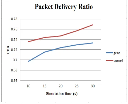
Packet delivery ratio is the ratio of the number of delivered data packet to the destination to the total number of packets originated from the source in the network. This illustrates the level of delivered data to the destination.
Table 1: Simulation Parameters
Number of nodes 371
Routing Protocols Geographic Routing
Dimensions of Topography 1024*100 m2
Packet Size 812
Channel Type Wireless Channel
Antenna Omni-directional
Antenna
Mac Protocol MAC 802_11
The Graph shows that the packet delivery ratio is increasing with simulation time, this indicates that proper delivery of data packets is taking place between source and destination node.
Fig 5. Packet Delivery Ratio Vs. Simulation Time
geographic routing algorithm. Thus from the simulated characteristics we can conclude that the CONSEL renders much better Packet Delivery as compared to geographic routing.
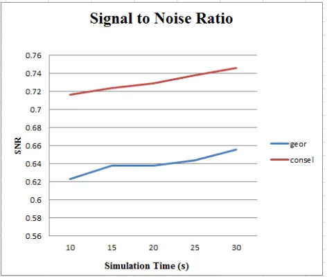
Fig 6. Signal-to-Noise Ratio Vs. Simulation Time
An important parameter while considering performance of a system is the Signal-to-Noise ratio, that is, the ratio of signal power to the noise power in the network. Higher signal to noise ratio is a good indictor implying good performance of the algorithm. The graph in figure 6 depicts the comparison of variation of signal to noise ratio with respect to simulation time for geographic routing assisted CONSEL and traditional geographic routing algorithm and it is evident that the signal to noise ratio is better for routing with the help of geographic routing assisted CONSEL algorithm.
Fig 7 Total Energy Consumption of Nodes Vs. Simulation Time
Energy consumption is another important parameter which is to be considered. Total energy consumption is the sum of energy spent in each node for transmission and reception in the network.
Initially, all the nodes in this network have sufficient battery power. Also, only little energy is consumed during the initial stages. But, as the simulation time is increased, and when more network activities are carried out naturally energy consumption increases.
The figure 7 shows the comparison of variation of the total energy consumed in the network with respect to simulation time for geographic routing assisted CONSEL and traditional geographic routing algorithm. The total energy consumption characteristics depicted indicates that the energy consumed during the operation is much lesser for CONSEL as compared to geographic routing.
5. Conclusion
Large scale 2D/3D sensor networks generally have complex irregular geometry, in which traditional algorithms does not exhibit optimum performance. The observed parameters such as like Packet Delivery Ratio (PDR), Signal-to-Noise Ratio, and energy consumption, from simulations of geographic routing as well as routing with help of CONSEL algorithm, indicated that traditional algorithms like geographic routing cannot be used to guarantee efficient routing in such large scale complex networks. The Greedy algorithms cannot resolve such dead-end or local minimum situation as in network concavities.
Even techniques like convex segmentation fails to deliver accurate results due to the dependence of the routing and localization techniques on concave node detection. The CONSEL is a scalable and distributed algorithm that segments the network based on connectivity information alone and performs routing and localization with better accuracy. With this technique traditional algorithms like greedy routing and geographic routing are adapted into a large scale complex 2-D/3-D environment.
Acknowledgment
References
[1] B.Karp and H.T.Kung, “GPSR: Greedy perimeter stateless routing for wireless networks,” in Proc. ACM MOBICOM, pp. 243–254, 2000.
[2] Savvides, C.Han, and M. B. Strivastava, “Dynamic fine-grained localization in ad hoc networks of sensors,” in Proc. ACM MOBICOM, pp. 166–179, 2001.
[3] T.K.Dey, J.Giesen, and S.Goswami, “Shape segmentation and matching with flow discretization,” in Proc. Workshop Algor. DataStruct., pp. 25– 36,2003.
[4] Panangadan and G.S.Sukhatme,“Data segmentation for region detection in a sensor network,” in Proc. DCOSS, pp. 1–12,2005.
[5] Xianjin Zhu, Rik Sarkar and Jie Gao “Topological Data Processing for Distributed Sensor Networks with Morse-Smale Decomposition” IJEIT Vol 2, No. 12, 2005.
[6] Stefan Funke " Topological Hole Detection in Wireless Sensor Networks and its Applications,"
DIALM-POMC'05, September 2005.
[7] Wenping Liu, Dan Wang, Hongbo Jiang, Wenyu Liu and Chonggang Wang “Approximate Convex Decomposition Based Localization in Wireless Sensor Networks” in Proc.National Nat-ural Science Foundation of China under Grant, 2006.
[8] X. Zhu, R. Sarkar, and J. Gao, “Shape segmentation and applications in sensor networks,” in Proc. IEEE INFOCOM, pp. 1838–1846, 2007.
[9] B.Leong, B. Liskov, and R. Morris, “Greedy virtual coordinates for geographic routing,” in Proc. IEEE ICNP, pp. 71–80, 2007.
[10] J.-M. Lien and N. M. Amato, “Approximate convex decomposition of polyhedra,” in Proc.ACM Symp.SolidPhys.Model, pp.121–131, 2007.
[11] J. Bruck, J. Gao, and A. A. Jiang, “Map: Medial axis based geometric routing in sensor networks,” in
Proc. Wireless Netw.,Vol.13, No.6, pp.835–853, 2007.
[12] Nguyen, N. Milosavljevic, Q. Fang, J. Gao, and L. J. Guibas, “Landmarkselection and greedy landmark-descent routing for sensor networks,” in Proc. IEEE INFOCOM, pp. 661–669, 2007.
[13] M. Li and Y. Liu, “Rendered path: Range-free localization in anisotropic sensor networks with holes,” in Proc. ACM MobiCom, pp. 51–62, 2007. [14] O.Saukh, R.Sauter, M.Gauger, P.J. Marron, and
K.Rothernel, “On boundary recognition without location information in wireless sensor networks,” in
Proc. IPSN, pp. 207–218, 2008.
[15] G. Tan, M. Bertier, and A.-M. Kermarrec, “Convex partition of sensor networks and its use in virtual coordinate geographic routing,” in Proc. IEEE INFOCOM, pp. 1746–1754, 2009.
[16] G. Tan, H. Jiang, S. Zhang, and A.-M. Kermarrec, “Connectivity-based and anchor-free localization in
large-scale 2D/3D sensor networks,” in Proc. ACM MobiHoc, pp. 191–200, 2010.
[17] Bi Jun Li, Min Jung Baek, Se Ung Hyeon, and Ki-Il Kim, “Load Balancing Parameters for Geographic Routing Protocol in Wireless Sensor Networks, ” in
Proc. IEEE INFOCOM, pp. 661–669, 2010.
[18] H. Zhou, N. Ding, M. Jin, S. Xia, and H. Wu, “Distributed algorithms for bottleneck identification and segmentation in 3D wireless sensor networks,” in Proc. IEEE SECON, pp. 494–502, 2011.
[19] H.Jiang, S.Jin, and C.Wang, “Predictionornot? An energy-efficient framework for clustering-based data collection in wireless sensor networks,” IEEE Trans. Parallel Distrib. Syst., Vol. 2, No. 6, pp.1064–1071, Jun. 2011.
[20] S. Xia, X. Yin, H. Wu, M. Jin, and X. D. Gu, “Deterministic greedy routing with guaranteed delivery in 3D wireless sensor networks,” in Proc. ACM MobiHoc, Art. no.1, 2011.
[21] Chi Zhang, Jun Luo, Liu Xiang, Feng Li, Juncong Lin and Ying He “Harmonic Quorum Systems: Data Management in 2D/3D Wireless Sensor Networks with Holes,” in Proc. AcRF Tier 2 Grant ARC15/11,
2011.
[22] Hongbo Jiang, Tianlong Yu, Chen Tian, Guang Tan and Chonggang Wang, “CONSEL: Connectivity-based Segmentation in Large-Scale 2D/3D Sensor Networks,” in Proc. IEEE INFOCOM, 2012.
[23] H. Jiang, S. Zhang, G. Tan, and C. Wang, “CABET: Connectivity-based boundary extraction of large-scale 3D sensor networks: Algorithm and Applications,” in Proc. IEEE INFOCOM, 2014.
Aparna K Menon completed her B.Tech in Electronics and Communication Engineering under Mahatma Gandhi University. Presently she is pursuing M.Tech in Electronics with specialization in Wireless Technology under Cochin University of Science and Technology(CUSAT).