University of Pennsylvania
ScholarlyCommons
Publicly Accessible Penn Dissertations
1-1-2014
Essays in Corporate Finance
Dieter Patrick Vanwalleghem
University of Pennsylvania, [email protected]
Follow this and additional works at:
http://repository.upenn.edu/edissertations
Part of the
Finance and Financial Management Commons
, and the
Sustainability Commons
This paper is posted at ScholarlyCommons.http://repository.upenn.edu/edissertations/1481
Recommended Citation
Vanwalleghem, Dieter Patrick, "Essays in Corporate Finance" (2014).Publicly Accessible Penn Dissertations. 1481.
Essays in Corporate Finance
Abstract
This dissertation examines the relationship between financial markets and firms' investment decisions. In particular, it focuses on three distinct settings in which firms' real and financial decisions are interconnected.
The first chapter looks at how firms' investment and savings decisions are affected by strategic interactions in their product markets. In particular, current dynamic models in corporate finance ignore the potential for strategic interactions between firms. Empirical evidence nevertheless suggests that these strategic interactions are present and influence corporate saving behavior in a non-trivial way. The first chapter proposes a dynamic model of imperfect competition which captures the empirical evidence and provides insight into how product market interactions influence and are influenced by corporate saving behavior.
The second chapter turns to socially responsible investment (SRI) and develops a micro-structure trading model which sheds new light on the relationship between SRI screening and a firms' equity cost of capital. Previous research argued that SRI screening will lead firms shunned by socially responsible investors to trade at a discount, i.e. have a higher cost or capital, relative to non-shunned peer firms. The model acknowledges this fact but also shows that asymmetric information and heterogeneity in beliefs regarding the relationship between corporate social and financial performance can dampen and even reverse the cost of capital gap between shunned and non-shunned firms. As such the model in the paper delivers a richer set of predictions which help explain the mixed empirical support for a link between SRI screening and equity cost of capital.
Finally, the third chapter outlines a new reason for why firms may finance themselves through financial contracts which provide explicit incentives to generate a social alongside a financial return on investment. The argument developed in this chapter does not rely on investor altruism nor on an explicit link between financial and corporate social performance. Instead it argues that social financial contracts can emerge naturally as the solution to a credit constraint problem in a common agency moral hazard setting. The paper predicts an inverted U-shape relationship between the use of social financial contracts and financial strength.
Degree Type
Dissertation
Degree Name
Doctor of Philosophy (PhD)
Graduate Group
Finance
First Advisor
Itay Goldstein
Keywords
Subject Categories
ESSAYS IN CORPORATE FINANCE
Dieter Vanwalleghem
A DISSERTATION
in
Finance
For the Graduate Group in Managerial Science and Applied Economics
Presented to the Faculties of the University of Pennsylvania
in
Partial Fulfillment of the Requirements for the
Degree of Doctor of Philosophy
2014
Supervisor of Dissertation
Itay Goldstein, Joel S. Ehrenkranz Family Professor, Professor of Finance
Graduate Group Chairperson
Eric T. Bradlow, K.P. Chao Professor, Professor of Marketing, Statistics and Education, Vice-Dean and Director of Wharton Doctoral Programs,
Co-Director of the Wharton Customer Analytics Initiative
Dissertation Committee
Itay Goldstein (Chair), Joel S. Ehrenkranz Family Professor, Professor of Finance
Mark Jenkins, Assistant Professor of Finance
ESSAYS IN CORPORATE FINANCE
c
COPYRIGHT
2014
Dieter Patrick Raymond Vanwalleghem
This work is licensed under the
Creative Commons Attribution
NonCommercial-ShareAlike 3.0
License
To view a copy of this license, visit
ACKNOWLEDGEMENT
I would like to thank my supervisors for their continuing support in the pursuit of my
doc-toral degree in Finance. Their advise and guidance have allowed me to push my intellectual
boundaries in writing the three papers comprising my dissertation.
Furthermore, I would like to thank my parents whose care and counsel were vital
through-out my entire eduction, but in particular during the years when I was working on my
dissertation.
Finally, I owe a great set of gratitude to my friends both at home and abroad who were
ABSTRACT
ESSAYS IN CORPORATE FINANCE
Dieter Vanwalleghem
Itay Goldstein
This dissertation examines the relationship between financial markets and firms investment
decisions. In particular, it focuses on three distinct settings in which firms real and financial
decisions are interconnected.
The first chapter looks at how firms investment and savings decisions are affected by
strate-gic interactions in their product markets. In particular, current dynamic models in
corpo-rate finance ignore the potential for stcorpo-rategic interactions between firms. Empirical evidence
nevertheless suggests that these strategic interactions are present and influence corporate
saving behavior in a non-trivial way. The first chapter proposes a dynamic model of
im-perfect competition which captures the empirical evidence and provides insight into how
product market interactions influence and are influenced by corporate saving behavior.
The second chapter turns to socially responsible investment (SRI) and develops a
micro-structure trading model which sheds new light on the relationship between SRI screening
and a firms equity cost of capital. Previous research argued that SRI screening will lead
firms shunned by socially responsible investors to trade at a discount, i.e. have a higher cost
or capital, relative to non-shunned peer firms. The model acknowledges this fact but also
shows that asymmetric information and heterogeneity in beliefs regarding the relationship
between corporate social and financial performance can dampen and even reverse the cost
of capital gap between shunned and non-shunned firms. As such the model in the paper
delivers a richer set of predictions which help explain the mixed empirical support for a link
Finally, the third chapter outlines a new reason for why firms may finance themselves
through financial contracts which provide explicit incentives to generate a social alongside
a financial return on investment. The argument developed in this chapter does not rely on
investor altruism nor on an explicit link between financial and corporate social performance.
Instead it argues that social financial contracts can emerge naturally as the solution to a
credit constraint problem in a common agency moral hazard setting. The paper predicts
an inverted U-shape relationship between the use of social financial contracts and financial
TABLE OF CONTENTS
ACKNOWLEDGEMENT . . . iv
ABSTRACT . . . v
LIST OF TABLES . . . viii
LIST OF ILLUSTRATIONS . . . ix
CHAPTER 1 : The strategic dimension of corporate cash . . . 1
1.1 Introduction . . . 1
1.2 Model . . . 5
1.3 Model solution . . . 12
1.4 Conclusion . . . 26
CHAPTER 2 : The real effects of socially responsible investing . . . 28
2.1 Introduction . . . 28
2.2 Model . . . 39
2.3 Model solution . . . 48
2.4 Analysis . . . 58
2.5 Conclusion . . . 69
CHAPTER 3 : Impact investing and social financial contracts . . . 72
3.1 Introduction . . . 72
3.2 Model . . . 87
3.3 Conclusion . . . 130
APPENDIX . . . 132
LIST OF TABLES
TABLE 1.1 : Baseline parameters . . . 14
TABLE 1.2 : Frequency table capital: base case . . . 21
TABLE 1.3 : Frequency table savings: base case . . . 22
TABLE 1.4 : Frequency table savings: base case, low market . . . 22
TABLE 1.5 : Frequency table savings: base case, medium market . . . 22
TABLE 1.6 : Frequency table savings: base case, high market . . . 23
TABLE 1.7 : Frequency table capital: λ0 = 0 . . . 23
TABLE 1.8 : Frequency table savings: λ0 = 0 . . . 23
TABLE 1.9 : Frequency table capital: λ1 = 0 . . . 24
TABLE 1.10 :Frequency table savings: λ1 = 0 . . . 24
TABLE 1.11 :Frequency table capital: λ1 = 0.05 . . . 24
TABLE 1.12 :Frequency table savings: λ1 = 0.05 . . . 25
TABLE 1.13 :Frequency table capital: φc=−0.1 . . . 25
TABLE 1.14 :Frequency table savings: φc=−0.1 . . . 25
LIST OF ILLUSTRATIONS
FIGURE 1.1 : Time Line . . . 5
FIGURE 1.2 : Profit plot . . . 15
FIGURE 1.3 : Capital policy strong firm . . . 17
FIGURE 1.4 : Capital policy weak firm . . . 18
FIGURE 1.5 : Marginal cost benefit analysis weak firm . . . 19
FIGURE 1.6 : Marginal cost benefit analysis strong firm . . . 20
FIGURE 2.1 : Timeline. . . 48
FIGURE 3.1 : Timeline . . . 89
FIGURE 3.2 : Social and non-social externality contract . . . 113
FIGURE 3.3 : Expected cost social financial contract . . . 122
FIGURE 3.4 : R1 bounds against ∆. . . 124
FIGURE 3.5 : R1 bounds againstB. . . 126
CHAPTER 1 : The strategic dimension of corporate cash
1.1. Introduction
1.1.1. Motivation
Traditionally, the notion of firms holding or hoarding cash has carried a negative
conno-tation. The view was that all available liquid assets should either be invested in physical
capital or, if no good investment opportunities are available, distributed to shareholders.
This view is partly rooted in the fear that large cash balances risk inducing managerial slack
and therefore destroy shareholder value. Moreover, a company’s equity investors seek to
get exposure to its production technology and business opportunities, not to the short term
interest rate which they can achieve themselves at much lower transaction costs. The steady
increase in corporate liquidity in the last two decades and in particular in the wake of the
recent financial crisis, however, seems to suggest that holding a liquid balance sheet might
have substantial virtues. Previous studies have suggested these virtues might come under
the form of protection against underinvestment, Riddick and Whited (2009) and Opler et al.
(1999), or even under the form of tax benefits for international firms.
In addition however, there is increasing evidence that cash has a strategic dimension and
offers substantial benefits through this channel. Managers for instance often justify their
cash hoarding behavior by referring to strategic flexibility vis--vis their industry competitors.
Rocco Landesman, the Broadway producer now running the National Endowment for the
Arts, once said:
“The key to life is having a sense of possibility and the best way to achieve that
is to carry no less than $ 10,000 in cash with you at all times. Cash gets you
deals, enables you to act quickly and helps you sleep at night”.
In addition to this anecdotal evidence, past empirical research has indicated that firms
their competitors, Haushalter et al. (2007). Others have argued that large cash balances
are often held as war chests out of which companies can fund competitive strategies in order
to gain market share, Fresard (2010). From a theoretical perspective however, the strategic
dimension of cash balances has received relatively little attention. Though a few static
models have been developed, firms’ strategic use of cash thus far has not been explored in
a dynamic setting.
The goal of this paper is to explore the strategic dimension of cash by examining in a
dynamic setting how competitive forces drive firms’ optimal cash policies and how in return
firm’s cash balances affect competitive behavior in the product market. The main tool used
to answer this question is a dynamic model of imperfect competition where firms compete,
invest and save in the presence of financial market imperfections
Before going into the model details, however, a quick summary is given regarding the ways
in which cash is thought to have a strategic dimension. There are mainly two ways in which
the literature has considered cash as potentially having a strategic dimension.
Firstly, holding cash might prevent a firm from falling behind its competitors when industry
wide investment opportunities present themselves. That is, if external financing is costly,
cash poor firms might not be able to fully invest in these opportunities allowing cash rich
firms to fill the gap and potentially take a leadership position. This risk of underinvestment
and loss of investment opportunities and market share to competitors is often referred to
as predation risk. Haushalter et al. (2007) provide empirical evidence that firms actively
manage predation risk by maintaining larger cash balances. Moreover, the effect of
pre-dation risk on cash holdings is stronger the larger the interdependence of a firm’s growth
opportunities with those of its rivals. In particular, controlling for standard determinants
of cash holdings such as profitability, leverage, etc. , firms tend to hold larger cash balances
in more concentrated industries, when their production technology is more similar to that
of rivals and in industries where firms’ growth opportunities, as measured by stock returns,
Secondly, large cash reserves can have strategic benefits in that they directly or indirectly
affect behavior in a firm’s product market. Bolton and Scharfstein (1990) for instance, argue
that financial market imperfections can give financially unconstrained firms the incentive to
prey on financially constrained firms by pursuing aggressive product market strategies. Cash
reserves are thus viewed as a war chests to fund competitive strategies such as aggressive
pricing or advertising. Furthermore, cash reserves might be beneficial as a signaling device
to deter rivals from entering a market or make capital expenditures Benoit (1984). Fresard
(2010) documents using a natural experiment that large cash balances are associated with
large future gains in market share. Moreover, this effect tends to be stronger for firms
facing financially weaker competitors and for industries where firms’ growth opportunities
are more interdependent.
1.1.2. Related literature
The model developed in this paper is novel from the perspective of two different strands
of economic literature namely that of industrial organization and of corporate finance. On
the one hand, in industrial organization, dynamic models of oligopolistic competition have
become increasingly popular since Pakes and McGuire (1994) developed their dynamic
industry model of imperfect competition. The model is based on a so called quality ladder
structure in which the competitive strength of a firm is captured by a single variable, quality.
Depending on the context of the model, a firm’s quality can be interpreted as product quality
resulting from accumulated R&D, a firms locked-in customers in a model with switching
costs or a firm’s physical capital in a Cournot model with capacity constraints. Naturally,
in any real industry a wide variety of both independent and correlated variables determine a
firm’s competitive strength, however the key idea is that quality captures the most important
of these. Besanko and Doraszelski (2004) for instance applies the Pakes and McGuire (1994)
framework to study industry capacity dynamics under various assumptions on the nature of
competition. In particular, he compares capacity constrained Cournot quantity competition
to Besanko and Doraszelski (2004) in that as in his paper, the industry considered here only
comprises two firms and abstracts away from entry and exit decisions by firms. The model
differs however in that it does not assume the quality ladder structure and considers not
only firms’ real but also financial decisions. Indeed, the absence of firms’ financial decisions
is a common feature among all dynamic models in industrial organization developed up to
this point. It is in this sense that the current model seeks to contribute to the existing
literature in industrial organization.
In corporate finance however, a rich literature on dynamic models in which firms make both
real and financial decisions has been developed in the last ten years. Hennessy and Whited
(2005) and Hennessy and Whited (2007) for instance analyze and estimate a dynamic
capi-tal structure choice model for firms making joint real and financial decisions. An important
contribution from these papers is that they highlight the importance of taking into account
financial market imperfections when interpreting firm investment and financing decisions.
Riddick and Whited (2009), develop a dynamic model of the firm to analyze firm’s
sav-ing behavior in the presence of financial market imperfections. The model developed in
this paper borrow heavily from theirs in that it assumes a very similar investment and
financial environment. It differs crucially however, in that in theirs and as in all other
dy-namic corporate finance models, the implicit assumption is made that firms either operate
in perfect competition or as stand-alone monopolists. In other words these models ignore
the possibility that strategic interactions between firms determine their optimal real and
financial decisions. As indicated above, however, empirical evidence suggests that
strate-gic interactions are an important determinant of firm policy and should therefore not be
neglected.
In sum, the dynamic duopoly model developed in this paper is new in the sense that it
can be viewed as either a dynamic industrial organization model where firms take both real
and financial decisions or a corporate finance model where strategic considerations affect
Hennessy and Whited (2007) than to Pakes and McGuire (1994), because I chose not to
adopt the Pakes and McGuire (1994) quality ladder set-up but rather stay closer to the
corporate finance tradition with investment defined as a continuous variable.
In what follows I will describe the model.
1.2. Model
1.2.1. Overview
The model has an infinite horizon and time is discrete. The economic agents are two
firms which periodically compete in the product market and make both real and financial
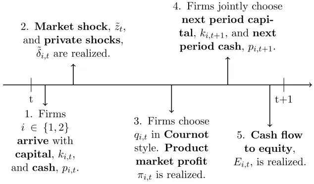
decisions. Figure 1.1 gives a chronological overview of the main events occurring in each
periodt.
t t+1
1. Firms i ∈ {1,2} arrive with
capital,ki,t, and cash,pi,t.
2. Market shock, ˜zt, and private shocks,
˜
δi,t are realized.
3. Firms choose qi,t in Cournot style. Product market profit
πi,t is realized.
4. Firms jointly choose
next period capi-tal,ki,t+1, and next
period cash,pi,t+1.
5. Cash flow to equity, Ei,t, is realized.
Figure 1.1: Time Line
At the beginning of each periodt, the two firms indexed byi∈ {1,2}arrive with an amount
of capital,ki,t and a level of cash holdings, pi,t carried over from the previous period. Both
firms publicly observe the realization of the market shock ˜zt and each firm privately learns
its depreciation shock ˜δi,t. Given the realization of the market shock and the firms’ capital
firm’s cost structure. In the product market competition phase, firms then simultaneously
choose their optimal production levels,qi,t, consistent with a Cournot quantity competition
equilibrium. The equilibrium production levels together with the market shock and the
capital levels then determine each firm’s profit from product market competition, πi,t.
Given this product market cash flow, both firms then simultaneously choose next period’s
optimal level of capital, ki,t+1, and the amount of cash, pi,t+1, to carry over to the next
period. In making these decisions firms realize that this pins down the cash flow to equity
Ei,t. Moreover, raising external equity capital is assumed to be costly in the model in that
negative realizations ofEi,t will command an extra cost per dollar of external equity raised.
In what follows each component of the model will be discussed in detail.
1.2.2. Product market Demand
The two firms are assumed to periodically compete in a market with no entry or exit. Each
firm produces one good and these goods are considered close substitutes in the eyes of the
consumer. One example of such a market is a market for new cars operated by two firms.
Though consumer preferences for one brand versus another create some form of market
power for each firm, consumers switch relatively easily to their less preferred brand should
that product be more readily available or offered at a lower price. The more substitutable
the goods are in the eyes of the consumer, the lower a firm’s market power and thus the
fiercer the competition. Intuitively, as the goods become more substitutable, each unit
produced by a firm’s competitor snaps away a bigger portion of a firm’s remaining market
potential.
The inverse demand function,P, facing firmi is given by:
Here, ˜zt ≥ 0 denotes the common market shock affecting both firms, φ0 < 0 is a firm’s
own inverse price elasticity of demand andφc<0 is a firm’s cross inverse price elasticity of
demand. The standard assumption for these type of demand functions is that |φc| ≤ |φ0|,
which implies that a firms own price matters more for its own demand than the price of its
competitor. High (low) absolute values ofφ0, imply that the firm faces an inelastic demand
in that large (small) increases in price are necessary to move the quantity demanded by the
firm’s consumers. φc on the other hand captures the degree of substitutability and hence
the strength of competition between the two firms. Higher (lower) absolute values of φc
imply that ceteris paribus, firm ihas to set a lower (higher) price in order to sell the same
number of units qi,t. In other words, A High (low) absolute value ofφccaptures the extent
to which the units sold a firm’s competitor reduce its own market potential.
1.2.3. Production technology
The production technology of each firm depends crucially on its level of capital, ki,t. In
particular, capital in the model determines a firm’s cost structure in that a higher level of
capital ceteris paribus implies lower production costs. Moreover, because the firms are
peri-odically engaged in Cournot quantity competition, capital is the primary strategic variable
in the model. This is because in Cournot competition a lower (higher) cost structure implies
a stronger (weaker) competitive position since firms with lower (higher) costs behave more
(less) aggressive. The easiest way to think of capital is accumulated R&D efforts in the
production process. The cost function, C(qi,t, ki,t) of both firms is given by:
C(qi,t, ki,t) =γqi,tαk β i,t.
Here α ≥ 1 implying that production costs are convex in the number of units produced.
Furthermore,β ≤0 capturing the negative relation between a firm’s level of capital and its
cost structure. Moreover, if |β|>1 the technology is increasing returns to scale, if|β|= 1
to scale. In the main solution of the model, it is assumed that |β|<1.
1.2.4. Static product market equilibrium
By combining the above demand function and the production technology we get that firm
i’s profit before financing costs and capital investments,π, is given by:
π(ki,t, kj,t,z˜t, qi,t, qj,t) =P(˜zt, qi,t, qj,t)qi,t−C(qi,t, ki,t).
The model as thus specifies exhibits a static dynamic break up which substantially simplifies
its computation. In particular, though the firm’s optimal investment and financing decisions
are dynamic decisions, made by taking into account their effect on future play, the optimal
optimal quantity, qi,t∗ , in each period is a static decision. To see this, note that a firm’s
quantity produced affects only its current product market profit and has no additional
dynamic implications. In particular, producing an output different from what is myopically
optimal does not affect a firm’s production capabilities in the future. It is for instance not
the case that a lower number of units produced implies a lower future rate of depreciation.
Given this static dynamic break-up, both firms can do no better than to choose the output
level that maximizes current period profits. Moreover, it is assumed that the firms
simul-taneously choose their quantities in a Cournot fashion so that the quantities produced are
assumed to be Cournot equilibrium quantities.
In particular givenk1,t, k2,t and ˜zt, the optimal quantities of both firms are the equilibrium
max q1,t
π(k1,t, k2,t,z˜t, q1,t, q2,t)
max q2,t
π(k2,t, k1,t,z˜t, q2,t, q1,t)
The per period profit before financing and investment then reduces to:
π∗(ki,t, kj,t,z˜t) =π(ki,t, kj,t,z˜t, q∗i,t, q∗j,t)
This greatly simplifies the model’s computation, because it implies that a reduced form
profit function π∗(ki,t, kj,t,z˜t) can be used when determining a firm’s optimal investment
and savings policies.
1.2.5. Capital investment
Each period, firms simultaneously choose how much to invest,xi,t, in their capital stockki,t.
Capital is subject to a one period time to build constraint and to stochastic depreciation.
In particular, each period firms receive a privately observed depreciation shock δi,t. One
can think of stochastic depreciation as the sum of constant periodic depreciation plus a
stochastic term reflecting unexpected machine failure, damage from fire,. . . etc. . This then
gives the following law of motion for capital:
ki,t+1 =xi,t+ (1−δ˜i,t)ki,t
1.2.6. Corporate saving
Shareholders in the model face an opportunity cost of funds equal tor. Each period firms
period’s cash balancepi,t+1. Corporate savings are invested in a one period risk-free bond
earning r(1−τ). This implies that the firm sets aside pi,t+1
r(1−τ) in period t to realize a cash
balance ofpi,t+1, next period. τ represents the cost of holding cash and is needed to ensure
firms in the model have bounded savings. This cost of holding cash can be interpreted in
several ways. For instance, the cost of cash could reflect an agency cost. This might arise
because large cash balances might make it harder to give proper incentives to the manager
of the firm to exert effort. An alternative interpretation is that holding cash implies a tax
cost because interest earned on internal savings is taxed at the corporate tax rateτc. For
simplicity this is the interpretation given to the cost of holding cash in this model. That is,
internal savings earn the risk free after tax returnr(1−τc).
1.2.7. Costly external finance
In any period t, if optimal investment and corporate savings exceed the cash flow from
product market competition and cash carried over from last period, the firm needs to raise
external equity capital. In the model, raising external equity capital is assumed to be costly
in that per dollar of external equity raised the firm incurs both a fixed cost λ0 >0 and a
variable cost of λ1 > 0 per dollar of external equity financing. The fixed equity issuance
costs can be interpreted as underwriting fees while the variable costs can be interpreted as
costs due to asymmetric information as in Myers and Majluf (1984).
1.2.8. Distribution to equity holders
Now we are in a position to define the periodic distribution to the shareholders. For ease
of notion, letsi,t ={ki,t, pi,t, kj,t, pj,t}. Then, firmi’s cash flow before financing is given by:
Π(si,t, si,t+1,˜zt,˜δi,t) =π∗(ki,t, kj,t,˜zt)−xi(ki,t+1, ki,t,δ˜i,t)
+pi,t−
pi,t+1
That is Π(si,t, si,t+1,z˜t,δ˜i,t) gives firmi’s cash flow before potential costs of rasing external
financing have been taken into account.
Let firm i’s cash flow to equity be denoted by E(si,t, si,t+1,z˜t,˜δi,t). The flow of funds
equation for firmi is then given by:
E(si,t, si,t+1,z˜t,δ˜i,t) = Π(si,t, si,t+1,z˜t,δ˜i,t)
−1[E<0]λ0−1[E<0]λ1|E(si,t, si,t+1,z˜t,δ˜i,t)|.
1.2.9. Value of the firm
Since shareholders discount future cash flows at the opportunity cost of funds r, the value
of firmiis given by:
Vi,t(si,t,z˜t,δ˜i,t) = max
{ki,t+u,pi,t+u}∞u=1 Et
"∞ X
u=0
E(si,t+u, si,t+u+1,z˜t+u,δ˜i,t+u) (1 +r)u
#
Or equivalently after rewriting in the Bellman form:
Vi(si,t,z˜t,δ˜i,t) = max ki,t+1,pi,t+1
E(si,t, si,t+1,z˜t,δ˜i,t) + 1 (1 +r)Et
h
Vi(si,t+1,z˜t+1,δ˜i,t+1)
1.2.10. Equilibrium of the dynamic game
The solution strategy for this model is to search for an equilibrium of the above dynamic
game. There are several equilibrium concepts that can be applied to this problem, but the
one that will be applied here is that of a Markov perfect equilibrium (MPE), Maskin and
Tirole (1988a) and Maskin and Tirole (1988b). The reason for choosing this equilibrium
concept is twofold. First, in terms of computation the MPE is by far the simplest to
compute because it allows the use of standard techniques in dynamic programming such as
value function iteration. Secondly, the Markov perfect equilibrium is also attractive from a
behavioral point of view in that it asserts that the equilibrium strategies of firms at point in
timetare a function only of a limited set of state variables. In particular, this implies that
the MPE does not consider equilibrium strategies that are path dependent. That is, all that
matters for the firms equilibrium strategies is the current state of the world as captured by
the state variables, s1,t,z˜t and ˜δ1,t and not how this state was reached.
In equilibrium, the optimal capital and savings policies of the two firms will then jointly
satisfy the system of Bellman equations:
V1(s1,t,z˜t,δ˜1,t) = max k1,t+1,p1,t+1
E(s1,t, s1,t+1,z˜t,˜δ1,t) + 1 (1 +r)Et
h
V1(s1,t+1,z˜t+1,˜δ1,t+1)
i
V2(s2,t,z˜t,δ˜2,t) = max k2,t+1,p2,t+1
E(s2,t, s2,t+1,z˜t,˜δ2,t) + 1 (1 +r)Et
h
V2(s2,t+1,z˜t+1,˜δ2,t+1)
i
1.3. Model solution
1.3.1. Model parameters
Due to the fact that this paper is the first dynamic corporate finance model to consider
strategic interactions between firms, the current literature provides very little guidance as
because the model borrows heavily from the set-up by Riddick and Whited (2009) with
regards to how a single firm is modelled in isolation, the approach taken in this paper
is to choose parameter values close to the ones used in their paper wherever possible.
As such, the only major difference in terms of parameter values between theirs and this
paper is with regards to the modeling of the market environment and the technology. In
particular, Riddick and Whited (2009) use a reduced form profit function, whereas in this
paper, the profit function is constructed from first principles. Nevertheless, in order to keep
the comparison as close as possible, the parameter values for the market and technology
parameters were chosen so as to mimic as closely as possible the behavior of a firms’ profits
as a function of its own capital. In particular, the parameter values on the technology yield
about the same range for a firm’s profits as a function of its own capital as in Riddick and
Whited (2009).
Profit parameters
The first component we need to describe is the process for the market shock ˜zt. This paper
follows Riddick and Whited (2009) in specifying that ˜zt follows an AR(1) in logs,
ln(˜zt) =ρln(˜zt−1) + ˜νt,
where ˜νt∼ N(0, σ2ν). The baseline parameter choices forρ and σν are respectively 0.8 and
0.25. To numerically solve the model, I need to specify a finite state space for the ˜zt. The
approach taken is to use Tauchen (1986) with 5 points on the state space with a range of
plus/minus 2 standard deviation shocks.
The own and cross price elasticities of demandφ0 andφcrespectively, are both set to -0.3 in
the baseline model. The fact that these two elasticities are equal, implies that the goods the
two firms produce will be considered closely substitutable by consumers. This will generate
equilibrium.
α in the model determines the behavior of a firm’s costs from operation for a given level of
capital. In the baseline case α is set to 1.6, which implies that the firm is facing a convex
cost function for a given level of capital ki,t. β, determines the impact of higher capital on
the cost structure of the firm. In the model, β is set to -0.85 reflecting a decreasing returns
to scale technology for the individual firm in that an increase in capital does not translate
into a one to one decrease in costs. Finally, γ is mainly used as a scaling parameter to
bring the level of costs in line with the level of revenues generated by ˜zt. γ is set to 2 in
our baseline computation.
These parameters taken together determine the reduced form profit function of a firm as
a function of its own and its competitors capital. Recall that this reduced form profit is
derived from assuming a Cournot equilibrium in quantities as outlined above in the model
discussion. As already mentioned, most of the baseline parameter values were chosen to
generate profit function behavior similar to that in Riddick and Whited (2009). In order
to give an idea of the behavior of the reduced form profit function of an individual firm,
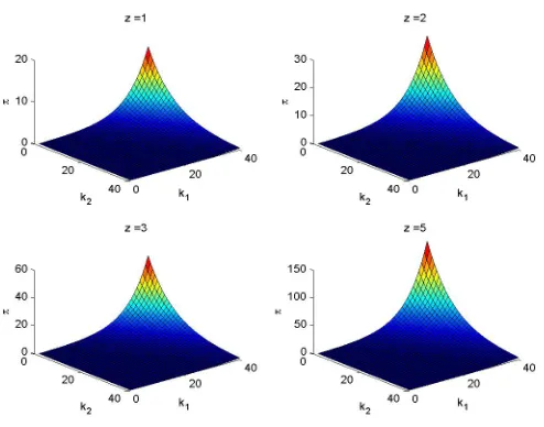
figure 1.2 plots profit, π, as a function of a firm’s own,k1 and its competitor’s, k2, capital
for 4 levels of the market shock, z. In figure 1.2, the numbers above the individual graphs
indicate the grid point for which the profit function was plotted, 1 indicating the lowest
level of z and 5 indicating the highest.
To summarize, the profit parameters in the baseline model are given in table 1.1:
parameter ρ σν ρ0 ρc α β γ
value 0.8 0.25 -0.3 -0.3 1.6 -0.85 2
Table 1.1: Baseline parameters
Investment parameters
The depreciation rate in the model, δi,t, is a privately observed random variable for each
Figure 1.2: Profit plot
in a given period is assumed to be a truncated normal random variable where the lower
truncation is set to 1 and the upper at Md. Each depreciation shock destroys δ of the
capital in place in going from one period to the next. In the baseline modelδ is set to 0.15
where M ud is set to 3. So the firm is subject at least to a depreciation rate of 0.15 and
can have a maximal depreciation rate of ≈0.52. The randomness in the depreciation rate
allows for the two firms to have distinct paths and hence for the possibility that one firm
will at some point trail or lead its competitor in terms of the level of capital. This will allow
for the possibility to determine whether firms are able to catch up with their competitor
under various scenarios of financial frictions.
Capital in the model is a choice variable and needs to be translated to a discrete state space.
In the baseline model, capital lies on a 40 point grid,
kmax(1−δ)39, kmax(1−δ)38, . . . , kmax(1−δ), kmax
Financial parameters
Finally, we need to specify the parameters governing the firm’s finances. First, the
oppor-tunity cost of funds in the model is set to 0.05. Secondly, the cost of holding cash τ is
assumed to be equal to the corporate tax rateτc and is set to 0.3. The cost of holding cash
is therefore interpreted as a tax related cost because internal savings of the firm are taxed
at the corporate tax rate. This will ensure the model exhibits bounded levels of corporate
savings.
The firm faces costly external financing under the form of a fixed,λ0and a variable,λ1 cost
of raising external equity financing. In the modelλ0 = 0.5 whileλ1 = 0.05. These values are
close to those chosen by Riddick and Whited (2009) except that their specification allows
for convex costs of external financing while in this model only linear costs are considered
for simplicity.
Lastly, savings in the model need to be translated to a discrete grid. In the baseline model,
corporate savings lie on a 5 point equally spaced grid from 0 to 5.
1.3.2. Baseline model results.
The model is solved using a modified policy function iteration approach. In each iteration,
first the capital and savings policies of the firm are updated using the value function in
memory and then in a second step the value function is converged upon fixing the
cap-ital and savings policies. This approach substantially improved the converge behavior of
the algorithm which can not rely on standard contraction mapping arguments that would
guarantee a convergence.
In order to give a flavor of the strategic behavior that firms exhibit in the model, consider a
state of the world in which a strong firm, w.l.o.g. here assumed to be firm 1, faces another
firm, firm 2. Competitive strength in the model is derived from two sources. On the one
in the product market. On the other hand, financial strength determines the ability of a firm
to respond cheaply to new investment opportunities that present themselves in the market.
Indeed, because raising external financing is costly, cash rich firms face a considerably lower
cost of investment than cash poor firms who have to rely on external financing. In what
follows, firm 1 is assumed to have a capital of k = 30 and a level of cash holding p = 4.
Firm 2’s capital and savings on the other hand are allowed to vary. This will allow us to
determine the impact of firm 2’s relative strength or weakness on the optimal capital policy
of firm 1.
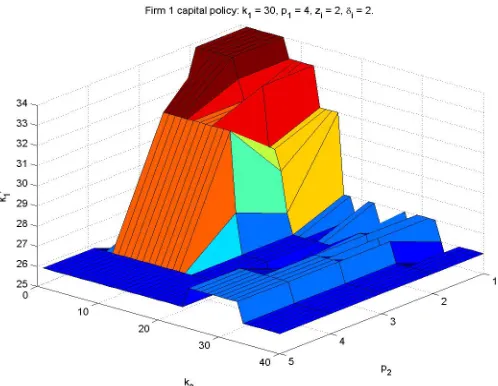
Figure 1.3: Capital policy strong firm
Figure 1.3 exhibits the capital policy of the strong firm 1, k10, as a function of the capital,
k2 and savings,p2 of firm 2. The policy function clearly indicates the predatory investment
behavior of firm 1 as its competitor becomes weaker both technologically and/or financially.
This is in line with Bolton and Scharfstein (1990) who indicate in a static model how similar
predatory behavior can emerge endogenously in a model of financial market imperfections.
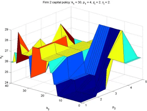
The same story but now from the perspective of firm 2 is featured in figure 1.4.
Figure 1.4 exhibits the optimal capital policy,k02, of firm 2 as a function of its own capital,
Figure 1.4: Capital policy weak firm
firm 2 becomes financially and technologically weaker, it is forced to scale back investment.
It is precisely this gap that firm 1 fills and hence results in firm 1 taking a leading position
in the industry. Notice that the capital difference between firm 1 and a weak firm 2 is
substantial, amounting to about 10 points on the capital grid.
In order to understand the fundamental factors driving these results figures 1.5 and 1.6
capture the trade-offs firm 1 and 2 make in determining their optimal capital policies. For
simplicity, assume that the fixed costs of external financing are zero.
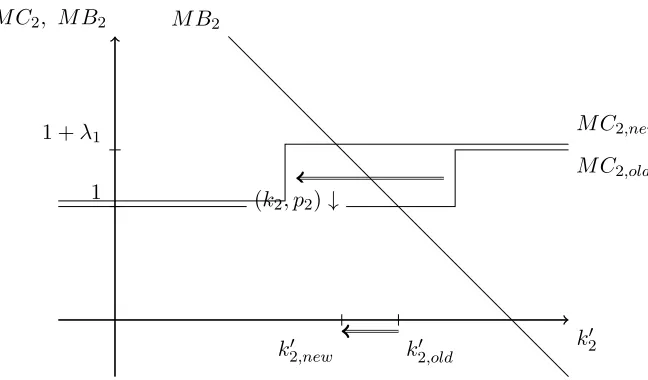
Figure 1.5 represents the marginal benefits and marginal costs for firm 2 of an additional
unit of next period capital as a function of the level of next period capital, k20. Naturally,
the optimal level of next period capital is determined where the marginal cost and marginal
benefit curves intersect. First let’s consider how to interpret the individual curves. The
marginal cost curve, M C2, is the easiest. The marginal cost of an extra unit of installed
capital at timet+ 1 is incurred at timet. For low levels of next period capital, the firm does
not have to tap the external financial markets and the cost of an extra dollar worth of next
period capital is simply one dollar. However, as the level of next period capital and thus
k20 M C2, M B2
M C2,old
1 (k
2, p2)↓
M C2,new 1 +λ1
M B2
k20,new k02,old
Figure 1.5: Marginal cost benefit analysis weak firm
point will have to start tapping into the external financial markets. This is the point where
the marginal cost function jumps upward from a level of 1 to a level of 1 +λ1 reflecting the
per dollar variable cost of external financing. The point at which the marginal cost curve
jumps upward is determined amongst other things by the level of internal cash available
which is in turn determined by the firm’s current level of capital,k2, and its current level of
savings, p2. As these variables decrease, the firm has less internal cash resources available
forcing it to seek external financing at lower levels ofk02. The marginal benefit of an extra
unit of capital is given by the downward sloping line M B2. This line is downward sloping
because of the assumption of decreasing returns to scale. Now consider what happens as
firm 2 becomes weaker financially and or in its level of capital. Initially, firm 2 has the
M C2,old marginal cost curve and the optimal level of next period capital is given by k20,old.
As firm 2 weakens its marginal cost curve shifts to the left to M B2,new reflecting the lower
level of internal cash resources. This reduces the optimal level of next period capital to
k02,new. As such the marginal benefit cost analysis in figure 1.5 captures the dynamics of
the policy function in figure 1.4.
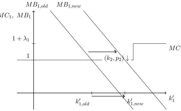
Now consider the optimal capital policy of the strong firm as it faces a competitor that
k01 M C1, M B1
M C1
1 1 +λ1
(k2, p2)↓
M B1,old M B1,new
k01,old k10,new
Figure 1.6: Marginal cost benefit analysis strong firm
the same as for the weak firm so won’t be repeated here. As firm 2 becomes financially and
or technologically weaker, the marginal benefits to firm 1 from an extra unit of installed
capital tomorrow increase as reflected by the shift from the marginal benefit curve from
M B1,old toM B1,new. The reason for this is that as firm 2 becomes weaker, firm 1 realizes
its competitor will optimally reduce its level of next period capital as outlined above. Firm
1 thus shifts its beliefs on firm 2’s next period capital to the lower end of the capital
distribution. However, the marginal benefits to a firm from an extra unit of installed
capital increase as its competitor chooses lower levels of future installed capital. This is
because the stronger firm now essentially has a larger market potential at its disposal. The
shift in the marginal benefits then results in an increase in the optimal level of next period
installed capital from k10,old tok01,new, reflecting the dynamics of figure 1.3.
1.3.3. Comparative statics results.
In this section, a comparative statics exercise for the baseline model is carried out. Because
this paper is primarily concerned with strategic interactions within a two firm or duopoly
market, the most interesting insights come from looking at the steady state industry
struc-ture. To obtain the steady state industry structure, a simulation based approach is taken
and savings’ behavior for, T = 100001 periods. Frequency tables then capture the fraction
of periods the industry finds itself in a given capital (savings) state. A capital (savings)
state is simply the level of capital (savings) chosen by firm 1 and firm 2 in a given periodt.
First, the steady state will be analyzed for the base case parameters outlined in the previous
section. In addition to the base case, a comparative statics exercise will be carried out by
considering four different parameter set ups. In particular, what will be considered are the
effects on the industry structure from changes in the cost of external financing, λ0 and λ1
respectively, and the intensity of competition, orφcrelative to φo.
One interesting question we will be able to answer from the steady state analysis is whether
the industry converges to a symmetric or asymmetric industry structure. The reason one
might believe an asymmetric industry structure might arise is that costly external
financ-ing, and especially the fixed cost of external financfinanc-ing, might prevent laggard firms in the
industry to catch up with the leader. Alternatively, costly external financing might not lead
to a steady state asymmetric industry structure but simply reduce the speed with which
the laggard firm catches up with the leader.
k2\k1 k1 (1−4) k 1 (5−8) k 1 (9−12) k 1 (13−16) k 1 (17−20) k 1 (21−24) k 1 (25−28) k 1 (29−32) k 1 (33−36) k 1 (37−40) k2
(1−4) 0.00 0.00 0.00 0.00 0.00 0.00 0.00 0.00 0.00 0.00
k2
(5−8) 0.00 0.00 0.00 0.00 0.00 0.00 0.00 0.00 0.00 0.00
k2
(9−12) 0.00 0.00 0.00 0.00 0.00 0.00 0.00 0.00 0.00 0.00
k2
(13−16) 0.00 0.00 0.00 0.00 0.00 0.00 0.00 0.00 0.00 0.00
k2
(17−20) 0.00 0.00 0.00 0.00 0.00 0.00 0.00 0.00 0.00 0.00
k2
(21−24) 0.00 0.00 0.00 0.00 0.00 0.06 0.00 0.00 0.00 0.00
k2
(25−28) 0.00 0.00 0.00 0.00 0.00 0.00 0.23 0.00 0.00 0.00
k2
(29−32) 0.00 0.00 0.00 0.00 0.00 0.00 0.00 0.00 0.00 0.00
k2
(33−36) 0.00 0.00 0.00 0.00 0.00 0.00 0.00 0.00 0.36 0.00
k2
(37−40) 0.00 0.00 0.00 0.00 0.00 0.00 0.00 0.00 0.00 0.35
Table 1.2: Frequency table capital: base case
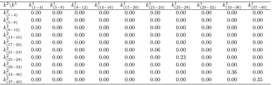
First consider the base case parameter set-up. Table 1.2 gives the frequency table for
industry capital in the steady state. Because the state space for capital contains,nk = 40,
points, the different capital states are grouped together by four for convenience. For instance
1
p2\p1 p11 p21 p13 p14 p15 p2
1 0.35 0.00 0.00 0.00 0.00
p2
2 0.00 0.03 0.00 0.00 0.00
p2
3 0.00 0.01 0.20 0.03 0.00
p2
4 0.00 0.00 0.02 0.35 0.00
p2
5 0.00 0.00 0.00 0.00 0.00
Table 1.3: Frequency table savings: base case
the cell (k(212 −24), k(211 −24)) indicates that 6% of the time the industry structure is such that
the capital levels of both firm 1 and firm 2 are between position 21 and 24 on the capital
grid. In general, table 1.2 indicates that the industry always converges to a symmetric
steady state in which capital is concentrated on the higher end of the capital grid.
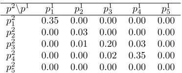
Similarly, table 1.3 gives the frequency table for industry savings in the steady state. This
indicates that industry savings is zero 35 % of the times and then concentrated around level
3 and 4 for the remainder of the time.
Note that the different sets of capital and savings concentrations in the above tables
cor-respond to the different states of the industry as captured by the market shock, z. To
illustrate this, tables 1.4 to 1.6 give industry savings in the steady state, but conditional on
whether the state of the market is low, table 1.4, intermediate, table 1.5, or high, table 1.6.
p2\p1 p1
1 p12 p13 p14 p15
p2
1 0.02 0.00 0.00 0.00 0.00
p22 0.00 0.02 0.00 0.00 0.00
p23 0.00 0.00 0.37 0.03 0.00
p24 0.00 0.00 0.02 0.54 0.00
p25 0.00 0.00 0.00 0.00 0.00
Table 1.4: Frequency table savings: base case, low market
p2\p1 p11 p21 p13 p14 p15
p2
1 0.21 0.00 0.00 0.00 0.00
p2
2 0.00 0.05 0.01 0.01 0.00
p2
3 0.00 0.03 0.19 0.04 0.00
p2
4 0.00 0.00 0.04 0.42 0.00
p2
5 0.00 0.00 0.00 0.00 0.00
Table 1.5: Frequency table savings: base case, medium market
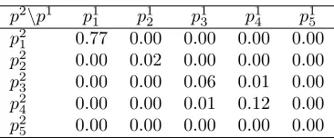
p2\p1 p11 p21 p13 p14 p15 p2
1 0.77 0.00 0.00 0.00 0.00
p2
2 0.00 0.02 0.00 0.00 0.00
p2
3 0.00 0.00 0.06 0.01 0.00
p2
4 0.00 0.00 0.01 0.12 0.00
p2
5 0.00 0.00 0.00 0.00 0.00
Table 1.6: Frequency table savings: base case, high market
they adjust their behavior to the increase (decrease) in investment opportunities. In tables
not reported here we find a similar picture for capital in that better market environments
lead both firms to choose a higher level of capital. Note also that even conditional on the
market environment there does not appear to be any indication of significant asymmetries
arising in the structure of the industry.
Now consider what happens when the cost of external financing is altered. Tables 1.7 to
1.12 represent the steady state levels of capital and savings in the industry for different
specifications of the external cost of financing. In particular, tables 1.7 and 1.8 represent
the situation where the fixed costs of raising equity capital, λ0, are set to zero.
k2\k1 k1 (1−4) k 1 (5−8) k 1 (9−12) k 1 (13−16) k 1 (17−20) k 1 (21−24) k 1 (25−28) k 1 (29−32) k 1 (33−36) k 1 (37−40) k2
(1−4) 0.00 0.00 0.00 0.00 0.00 0.00 0.00 0.00 0.00 0.00
k2
(5−8) 0.00 0.00 0.00 0.00 0.00 0.00 0.00 0.00 0.00 0.00
k2
(9−12) 0.00 0.00 0.00 0.00 0.00 0.00 0.00 0.00 0.00 0.00
k2
(13−16) 0.00 0.00 0.00 0.00 0.00 0.00 0.00 0.00 0.00 0.00
k2
(17−20) 0.00 0.00 0.00 0.00 0.00 0.00 0.00 0.00 0.00 0.00
k2
(21−24) 0.00 0.00 0.00 0.00 0.00 0.08 0.00 0.00 0.00 0.00
k2
(25−28) 0.00 0.00 0.00 0.00 0.00 0.00 0.21 0.00 0.00 0.00
k2
(29−32) 0.00 0.00 0.00 0.00 0.00 0.00 0.00 0.02 0.01 0.00
k2
(33−36) 0.00 0.00 0.00 0.00 0.00 0.00 0.00 0.01 0.33 0.00
k2
(37−40) 0.00 0.00 0.00 0.00 0.00 0.00 0.00 0.00 0.00 0.34
Table 1.7: Frequency table capital: λ0= 0
p2\p1 p1
1 p12 p13 p14 p15
p2
1 0.85 0.00 0.00 0.00 0.00
p2
2 0.00 0.15 0.00 0.00 0.00
p2
3 0.00 0.00 0.00 0.00 0.00
p2
4 0.00 0.00 0.00 0.00 0.00
p2
5 0.00 0.00 0.00 0.00 0.00
Table 1.8: Frequency table savings: λ0 = 0
costs, which is in line with what is documented by Riddick and Whited [2006]. In 85 % of
the periods, both firms hold no cash compared to only 35 % of the periods in the presence
of fixed costs. On the other hand, setting the fixed costs to zero has virtually no discernible
effect on capital as indicated by table 1.7.
k2\k1 k1
(1−4) k(5−8)1 k1(9−12) k1(13−16) k1(17−20) k1(21−24) k1(25−28) k1(29−32) k1(33−36) k1(37−40)
k2
(1−4) 0.00 0.00 0.00 0.00 0.00 0.00 0.00 0.00 0.00 0.00
k2
(5−8) 0.00 0.00 0.00 0.00 0.00 0.00 0.00 0.00 0.00 0.00
k2
(9−12) 0.00 0.00 0.00 0.00 0.00 0.00 0.00 0.00 0.00 0.00
k2
(13−16) 0.00 0.00 0.00 0.00 0.00 0.00 0.00 0.00 0.00 0.00
k2
(17−20) 0.00 0.00 0.00 0.00 0.00 0.00 0.00 0.00 0.00 0.00
k2
(21−24) 0.00 0.00 0.00 0.00 0.00 0.07 0.00 0.00 0.00 0.00
k2
(25−28) 0.00 0.00 0.00 0.00 0.00 0.00 0.25 0.00 0.00 0.00
k2
(29−32) 0.00 0.00 0.00 0.00 0.00 0.00 0.00 0.00 0.01 0.00
k2
(33−36) 0.00 0.00 0.00 0.00 0.00 0.00 0.00 0.01 0.33 0.00
k2
(37−40) 0.00 0.00 0.00 0.00 0.00 0.00 0.00 0.00 0.00 0.32
Table 1.9: Frequency table capital: λ1= 0
p2\p1 p1
1 p12 p13 p14 p15
p2
1 0.42 0.01 0.00 0.00 0.00
p22 0.01 0.34 0.00 0.00 0.00
p23 0.00 0.01 0.01 0.02 0.00
p24 0.00 0.00 0.02 0.16 0.00
p25 0.00 0.00 0.00 0.00 0.00
Table 1.10: Frequency table savings: λ1 = 0
k2\k1 k1 (1−4) k 1 (5−8) k 1 (9−12) k 1 (13−16) k 1 (17−20) k 1 (21−24) k 1 (25−28) k 1 (29−32) k 1 (33−36) k 1 (37−40) k2
(1−4) 0.00 0.00 0.00 0.00 0.00 0.00 0.00 0.00 0.00 0.00
k2
(5−8) 0.00 0.00 0.00 0.00 0.00 0.00 0.00 0.00 0.00 0.00
k2
(9−12) 0.00 0.00 0.00 0.00 0.00 0.00 0.00 0.00 0.00 0.00
k2
(13−16) 0.00 0.00 0.00 0.00 0.00 0.00 0.00 0.00 0.00 0.00
k2
(17−20) 0.00 0.00 0.00 0.00 0.00 0.00 0.00 0.00 0.00 0.00
k2
(21−24) 0.00 0.00 0.00 0.00 0.00 0.07 0.00 0.00 0.00 0.00
k2
(25−28) 0.00 0.00 0.00 0.00 0.00 0.00 0.24 0.00 0.00 0.00
k2
(29−32) 0.00 0.00 0.00 0.00 0.00 0.00 0.00 0.01 0.00 0.00
k2
(33−36) 0.00 0.00 0.00 0.00 0.00 0.00 0.00 0.00 0.37 0.00
k2
(37−40) 0.00 0.00 0.00 0.00 0.00 0.00 0.00 0.00 0.00 0.32
Table 1.11: Frequency table capital: λ1 = 0.05
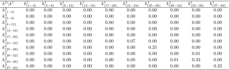
In contrast to lowering the fixed cost of external capital, tables 1.9 to 1.12 indicate that
lowering the variable cost of external financing has very little effect on optimal level of
savings and capital in the industry. Though savings is somewhat reduced asλ1 is lowered,
p2\p1 p11 p21 p13 p14 p15 p2
1 0.32 0.00 0.00 0.00 0.00
p2
2 0.00 0.04 0.01 0.01 0.00
p2
3 0.00 0.02 0.18 0.04 0.00
p2
4 0.00 0.00 0.03 0.36 0.00
p2
5 0.00 0.00 0.00 0.00 0.00
Table 1.12: Frequency table savings: λ1 = 0.05
That is the fixed costs of external financing are the crucial driver of the precautionary
savings motive in the model.
k2\k1 k1 (1−4) k 1 (5−8) k 1 (9−12) k 1 (13−16) k 1 (17−20) k 1 (21−24) k 1 (25−28) k 1 (29−32) k 1 (33−36) k 1 (37−40) k2
(1−4) 0.00 0.00 0.00 0.00 0.00 0.00 0.00 0.00 0.00 0.00
k2
(5−8) 0.00 0.00 0.00 0.00 0.00 0.00 0.00 0.00 0.00 0.00
k2
(9−12) 0.00 0.00 0.00 0.00 0.00 0.00 0.00 0.00 0.00 0.00
k2
(13−16) 0.00 0.00 0.00 0.00 0.00 0.00 0.00 0.00 0.00 0.00
k2
(17−20) 0.00 0.00 0.00 0.00 0.00 0.00 0.00 0.00 0.00 0.00
k2
(21−24) 0.00 0.00 0.00 0.00 0.00 0.06 0.00 0.00 0.00 0.00
k2
(25−28) 0.00 0.00 0.00 0.00 0.00 0.00 0.19 0.00 0.00 0.00
k2
(29−32) 0.00 0.00 0.00 0.00 0.00 0.00 0.00 0.00 0.00 0.00
k2
(33−36) 0.00 0.00 0.00 0.00 0.00 0.00 0.00 0.00 0.35 0.00
k2(37−40) 0.00 0.00 0.00 0.00 0.00 0.00 0.00 0.00 0.00 0.39
Table 1.13: Frequency table capital: φc=−0.1
p2\p1 p1
1 p12 p13 p14 p15
p2
1 0.40 0.00 0.00 0.00 0.00
p2
2 0.00 0.03 0.02 0.00 0.00
p2
3 0.00 0.02 0.16 0.01 0.00
p2
4 0.00 0.00 0.03 0.33 0.00
p2
5 0.00 0.00 0.00 0.00 0.00
Table 1.14: Frequency table savings: φc=−0.1
Finally, tables 1.13 and 1.14 capture a novel result not documented by previous dynamic
models in corporate finance. In particular, tables 1.13 and 1.14 indicate how a change in
the strength of competitive interactions between firm 1 and 2 change their optimal capital
and savings policies. In tables 1.13 and 1.14, the financial parameters are as in the base case
model, but the strength of competitive interaction is reduced by lowering the cross price
elasticity parameter,φo, from -0.3 to -0.1. In practice this means that both firms have more
market power in their own market segment and hence have to worry less about consumers
effect on savings is that both firms lower their savings when competition is reduced. That
is the industry savings distribution shifts to lower levels of savings. This indicates that
conditional on costly external financing, firms hold lower cash balances when the level of
competition is reduced. This is explained by the fact that predatory investment behavior
is less profitable when the firms are more distinct in the eyes of the consumer, i.e. lower
φo, so that the firms have less incentives to build up a cash buffer to ensure competitive
viability in the future.
1.4. Conclusion
Dynamic models of firm financial decision making have received increasing attention in
recent years. These models however, usually depart from either monopolistic or perfect
competition and thus ignore the effect strategic considerations might have on firms’ optimal
real and financial policies. Moreover, empirical evidence suggests that strategic interactions
between firms are indeed present and have a non trivial impact on firms’ financial decisions
and in particular on their cash holding strategies. In a dynamic duopoly model of the
firm, this paper documents the tendency for financially strong firms to prey on weaker
firms by investing aggressively in an attempt to capture market share of their competitor.
This threat of predation by competitor firms generates a precautionary motive for hoarding
cash not present in monopolistic models or models of perfect competition. In particular,
the model indicates that controlling for the cost of external financing, as the strength of
competitive interaction increases, firms in the industry tend to hold larger cash balance
on average. Another interesting feature of the model is that costly external financing does
note appear to be able to endogenously generate an asymmetric industry structure. In other
words, costly external financing does not prevent laggards in the industry to catch up with
the leader. All results in this paper however are based on a rather loose parameterization
as the current literature provides little guidance as to how to set the various parameters in
the model. An interesting question for future research would therefore be to estimate the
Whited (2005). This exercise would be particularly valuable with respect to the competition
parameters, since for these parameters little guidance was available and the results show
CHAPTER 2 : The real effects of socially responsible investing
2.1. Introduction
2.1.1. Motivation
Socially responsible investment (SRI) has become an increasingly popular investment
prac-tice in recent years. The US Social Investment Forum (USSIF), a national not-for-profit
organization that promotes the concept, practice and growth of socially responsible
invest-ing, reports that in 2010 12.2 % of the $25.2 trillion in total assets under management
tracked by Thomson Reuters Nelson is involved in some strategy of socially responsible
investing.
One of the primary goals of SRI is to allow consumers to align their investment savings
decisions with their personal values and its most popular application at the moment is
the use of socially responsible investment screens. These investment screens are applied
within otherwise standard financial investment analysis and effectively reduce the universe
of stocks to a subset of shares who are deemed morally or ethically acceptable to socially
responsible investors.
Broadly speaking, a socially responsible investment screen is a set of environmental, social
or ethical criteria which determine which shares are eligible for trade to an investor who
wishes to invest only in firms whose practices and policies are in line with his personal
values. As such the portfolio allocation decisions of socially responsible investors are a
function of not only financial but also non-financial factors reflecting the personal attitude
of these investors towards certain corporate practices and policies.
Advocates of SRI however claim that SRI screens are more than a mere tool allowing
investors to meet their moral obligations towards investing. In particular they argue that by
selectively investing in firms exhibiting a high corporate social performance (CSP) socially
improve their CSP.
Research in finance examining this claim about the real effects of SRI however is scarce
and therefore relatively little is known about its validity. This is unfortunate since research
in finance is increasingly examining how financial markets feed back into the investment
decision by firms as evidenced for instance by work by Chen et al. (2007) and Bond et al.
(2012). By analyzing SRI, a new channel through which financial markets determine firm
investment decisions can therefore be explored.
The goal of this paper is to partly fill this gap in the literature by revisiting the question
on equilibrium equity cost of capital formation when the financial market is populated by
socially responsible investors. Socially investors differ from traditional investors in two
ways.
First, socially responsible investors apply SRI screens and invest only in firms which exhibit
a high CSP.
Secondly, socially responsible investors believe that firms with a higher CSP also have a
higher corporate financial performance (CFP). This so called “doing well while doing good”
hypothesis is currently hotly debated in both professional and academic circles.
Nevertheless many SRI practitioners claim that the screening of firms on their CSP not
only allows them to selectively invest in virtuous firms but also that it unearths valuable
insights into firms’ competitiveness and profitability. As such socially responsible investors
can be expected to condition their trades above and beyond the screening outcome on this
additional piece of information about a firm’s fundamental.
Previous research which looked into the effects of socially responsible investors on a firm’s
equilibrium cost of capital, primarily focussed on the impact of SRI screening, Angel and
Rivoli (1997) and Heinkel et al. (2001). This paper adds to the existing literature by not
active trading of socially responsible investors on information related to the firm’s corporate
social performance.
Moreover, traditional investors are assumed to not to trade on this CSP information
be-cause they regard it as irrelevant. As such socially responsible and traditional investors
are assumed to openly disagree on the cash flow importance of a firm’s corporate social
performance.
The main point this paper will then seek to make is that although SRI screens have the
potential to lower the cost of capital of firms with a high CSP, this need not be the case
if socially responsible investors trade on and disagree with traditional investors about the
importance of CSP information.
The reason for this is that although trading on so called environmental, social and
gov-ernance (ESG) information, which captures corporate social performance, has gained
mo-mentum among investors, it is primarily socially responsible investors who are leading this
trend. Most traditional investors still dismiss the relevance of ESG risks and
opportuni-ties and hence largely ignore it as a source of information on the firm’s future cash flow
performance.
This apparently open disagreement between traditional and socially responsible investors on
the importance of CSP information is what might lead the investment strategies of socially
responsible investors to harm the cost of capital of high CSP firms or to at least make
the cost of capital gap between high and low CSP firms to be smaller than what standard
theory in finance might predict.
In particular, socially responsible investment screens imply that high CSP firms will have a
larger investor base than low CSP firms, all else equal, because the former are more likely to
be included into the portfolios of socially responsible investors. Standard theory in finance
then predicts that in a simple economy with risk averse investors, high CSP firms will enjoy
In a Grossman and Stiglitz (1980) economy with open disagreement on the value of CSP
information this argument still holds, but needs to be complemented by the fact that
tradi-tional investors will perceive the trading by socially responsible investors on CSP
informa-tion as an addiinforma-tional source of noise trading. If tradiinforma-tional investors are not fully informed
on this CSP noise such that they can not fully anticipate the effects on the equilibrium
share price, they will charge a risk premium for trading the shares of high CSP firms which
might offset the discount these firms enjoys because of their larger investor base.
This negative externality on the risk premium charged however is not the only effect the
open disagreement has on a firm’s cost of capital. In particular, in addition to the above
risk compensation channel, open disagreement affects a firm’s equilibrium cost of capital
through a mean return channel. The effect will moreover be positive or negative depending
on what the true underlying relationship is between CSP and CFP, that is whether the
beliefs of socially responsible or of traditional investors are correct.
For instance, if in reality CSP has no effect on the firm’s CFP yet socially responsible
investors believe there is, then their trading generates an additional demand for the shares
of high CSP firms which is reflected in the equilibrium price but not in the expectation
of the firm’s fundamental. This will lead a high CSP firm’s cost of capital to be too low
relative to what it should be.
On the other hand, if socially responsible investors are correct in their beliefs, then a high
CSP firm’s cost of capital will be too high relative to what it should be. This is because
although the firm’s fundamental will now fully reflect the CSP - CFP relationship, the
equilibrium price will only partly do so since only socially responsible investors incorporate
the true relationship into the equilibrium price.
The arguments put forward in this paper might therefore shed some light on why it has been
hard to find empirical evidence on the impact of socially responsible investment strategies
Future empirical research might then be guided by the propositions in this paper in order
to see whether corporate social performance effect on firms’ cost of capital can be identified.
In addition, the paper has implications for policy makers who want to stimulate socially
responsible investing as a mechanism to make firms internalize environmental or social
externalities. In particular, if traditional and socially responsible investors continue to
dis-agree on the relevance of CSP information, then the screening efforts by socially responsible
investors can be rendered less effective or even ineffective as a tool to make make firms
internalize their externalities via the cost of capital channel. For socially responsible
invest-ment screens to be more effective, policy makers need to control as much as possible the
noise premium charged by traditional investors.
The noise premium however is a result of traditional investors being less informed than
socially responsible investors about the firm’s CSP. If traditional investors were equally
well informed, they would be able to filter out the impact of socially responsible investor’s
trading activities on the equilibrium price. CSP information would then no longer appear
as a source of noise for traditional investors in the price signal and they would no longer
charge an additional noise premium.
In the next section an overview will be given of the current state of the socially responsible
investment sector. Following that, there will be a brief discussion of past research on socially
responsible investing in the finance literature.
2.1.2. Socially responsible investment sector
Socially responsible investing in the United States has experienced strong growth in the last
15 years. Growing substantially faster than the broader universe of conventional investment
assets under professional management, table 2.1 reports that assets following SRI strategies
grew from $639 billion in 1995 to $ 3.07 trillion in 2010. This represents a growth of 380
% in just over 15 years. Furthermore, during the recent financial crises, from 2007 to 2010,