Download Download PDF

doi:10.5556/j.tkjm.50.2019.2831

--++ ---

-A VISCOSITY ITER-ATIVE -ALGORITHM TECHNIQUE

FOR SOLVING A GENERAL EQUILIBRIUM PROBLEM SYSTEM

MASOUMEH CHERAGHI, MAHDI AZHINI AND HAMID REZA SAHEBI

Abstract. In the recent decade, a considerable number of Equilibrium problems have been solved successfully based on the iteration methods. In this paper, we suggest a vis-cosity iterative algorithm for nonexpansive semigroup in the framework of Hilbert space. We prove that, the sequence generated by this algorithm under the certain conditions im-posed on parameters strongly convergence to a common solution of general equilibrium problem system. Results presented in this paper extend and unify the previously known results announced by many other authors. Further, we give some numerical examples to justify our main results.

1. Introduction

The viscosity iterative algorithms for finding a common element of the set of fixed points for nonlinear operators and the set of solutions of variational inequality problems have been investigated by many authors [11,21,24,26,27] and references therein. The viscosity tech-nique for nonexpansive mappings in Hilbert space was proposed by Moudafi[9, 10]. This technique allow us to apply this method to convex optimization, linear programming and monoton inclusions [15,17,20,22,23,25]. It is well known that the generalized equilibrium problems include variational inequality problems, optimization problems, problems of Nash equilibria, saddle point problems, fixed point problems and complementarity problems as special cases [1,9,22,23].

LetC be a nonempty closed convex subset of a real Hilbert spaceHwith inner product

〈·,_·〉and norm_{k · k}. AmappingT :C_→C is said to be contraction if there exists a constant

α_∈(0, 1) such thatkT(x)−T(y)k ≤α_kx−yk,∀x,y∈C. Ifα₌1Tis called nonexpansive onC. The generalized equilibrium problem (GEP) is defined as follows:

Find x¯_∈C: F( ¯x,y)_{+ 〈}Ax¯,y₋x¯_{〉 ≥}0 _∀y_∈C, (1.1) 2010Mathematics Subject Classification. Primary : 47H09, 47H10; Secondary : 47J20.

Key words and phrases. Generalized equilibrium problem, fixed point problem, nonexpansive semi-group, strongly positive linear bounded operator, α-inverse strongly monotone mapping, Hilbert space.

Corresponding author: Mahdi Azhini.

whereA:C→His a nonlinear mapping, andF:C×C→Ris a bifunction. The set of solutions this problem is denoted by GEP(F,A)., i.e.,

GEP(F,A)={ ¯x∈C: F( ¯x,y)+ 〈Ax¯,y−x¯〉 ≥0, ∀y∈C}, which was studied by Takahashi [23].

To study the generalized equilibrium problem (1.1), we may assume thatF satisfies the following conditions:

(A1) F(x,x)≥0, ∀x∈C,

(A2) Fis monotone, i.e.F(x,y)+F(y,x)≤0, ∀x∈C, (A3) Fis upper hemicontinuouse, i.e. for eachx,y,z∈C,

lim sup

t_→0

F(t z₊(1₋t)x,y)_≤F(x,y),

(A4) For eachx_∈Cfixed, the functionx_→F(x,y) is convex and lower semi-continuous; A familyS:₌{T(s) : 0_≤s_{< ∞}} of mapping fromC into itself is called a nonexpansive semi-group onCif it satisfies the following conditions:

(1) T(0)x=xfor allx∈C,

(2) T(s+t)=T(s)T(t) for alls,t≥0,

(3) kT(s)x−T(s)yk ≤ kx−ykfor allx,y∈Cands≥0, (4) For allx_∈C,s_→T(s)xis continuous.

Plubtieng and Punpaeng introduced the following iterative method for nonexpansive semigroup[13]:

xn₊1=αnf(xn)+βnxn+(1−αn−βn)

1

sn

Zsn

0

T(s)xnd s.

In 2010 Kang et.al, introduced and inspired by results in [6], prove a strong convergence of the iterative scheme in a real Hilbert space by

xn₊1=αnγf(xn)+βnxn+((1−βn)I−αnA)

1

sn

Zsn

0

T(s)xnd s,

whereAis a strong positive bounded linear operator onC.

Cianciaruso et al. [3] considered the following iterative method:

F(un,y)+

1

rn〈

y₋un,un−xn〉 ≥0;

xn₊1=αnγf(xn)+(1−αnA)

1

sn

Zs_n

0

T(s)und s.

fixed points of a nonexpansive semigroup in a Hilbert space. They proved, under the certain appropriate conditions, the iterative algorithm converges strongly to the unique solution of a variational inequality. In this paper, by intuition from [3,6,13,14,15,16,17] a new iterative algorithm scheme is introduced. The results presented in this paper generalize, improve and unify many previously known results in this research area.

2. Preliminaries

For each pointx_∈H, there exists a unique nearest point ofC, denote byPCx, such that

kx₋PCxk ≤ kx−ykfor all y ∈C. PC is called the metric projection ofH ontoC. It is well

known thatPCis nonexpansive mapping and is characterized by the following property:

〈x₋PCx,y−PCy〉 ≤0 (2.1)

Definition 2.1. A mappingT :H→His said to be firmly nonexpansive, if

〈T x−T y,x−y〉 ≥ kT x−T yk2, ∀x,y∈H. Definition 2.2. A mappingM:C_→His said to be monotone, if

〈M x₋M y,x₋y_{〉 ≥}0, _∀x,y_∈C.

Mis calledα-inverse-strongly-monotone if there exist a positive real numberαsuch that

〈M x₋M y,x₋y_{〉 ≥}α_kM x₋M y_k2, _∀x,y_∈C.

Definition 2.3. A mappingB:H→His said to be strongly positive linear bounded operator, if there exists a constant ¯γ_>0 such that_〈B x,x_{〉 ≥}γ¯_kx_k2,_∀x_∈H.

Notation. Let {xn} be a sequence in H, then xn →x (respectively, xn *x) denote strong

(respectively, weak) convergence of the sequence {xn} to a pointx∈H.

It is known thatHsatisfies Opial’s condition [12], i.e., for any sequence {xn} withxn*x

the inequality

lim inf

n→∞ kxn−xk <lim infn→∞ kxn−yk (2.2)

holds for everyy∈Hwithy6=x.

Lemma 2.4([5]). Let C be a nonempty, closed convex subset of H and let F :C_×C _→Rbe a bifunction satisfying (A1)−(A4). Then For r>0and x∈H , there exists z∈C such that F(z,y)+

1

r〈y−z,z−x〉 ≥0, ∀y∈C . Further define

T_rFx₌{z_∈C:F(z,y)₊1

(i) T_rFis single-valued.

(ii) T_rFis firmly nonexpansive, i. e.,

kT_rF(x)₋T_rF(y)_k2_{≤ 〈}T_rF(x)₋T_rF(y),x₋y_〉, _∀x,y_∈H.

(iii) Fix(TrF)=EP(F).

(iv) EP(F)is compact and convex.

Lemma 2.5([4]). Let F :C_×C_→Rbe a bifunction satisfying(A1)₋(A4)and let T_rFbe defined as in Lemma2.4, for r_>0. Let x,y_∈H and r1,r2>0. Then,

kTrF2y−T

F

r1xk ≤ kx−yk + |

r2−r1

r2 |k

TrF2y−yk.

Lemma 2.6([8]). Assume that B is a strong positive linear bounded self adjoint operator on a Hilbert space H with coefficientγ¯_>0and0_<ρ_{≤ k}B_k−1_{. Then}

kI₋ρB_{k ≤}1₋ργ¯.

Lemma 2.7([18]). Let C be a nonempty bounded closed convex subset of a Hilbert space H and let S:={T(s) : 0≤s< ∞}be a nonexpansive semigroup on C , for each x∈C and t>0. Then, for any0≤h< ∞,

lim

t→∞supx_∈Ck

1

t

Zt

0

T(s)xd s−T(h)(1

t

Zt

0

T(s)xd s)k =0.

Lemma 2.8([19]). Let{xn}and{yn}be bounded sequences in a Banach space X and{βn}be a sequence in[0, 1]with0_<lim infn→∞βn≤lim supn_→∞βn<1. Suppose xn+1=(1−βn)yn+

βnxn, for all integers n≥0andlim sup

n→∞

(_kyn+1−ynk−kxn+1−xnk)≤0. Then_nlim

→∞kyn−xnk =0.

Lemma 2.9([23]). Let F:C_×C_→Rbe a bifunction satisfying(A1)₋(A4)and let T_rFbe defined as in Lemma2.4, for r_>0. Let x_∈H and s,t_>0. Then,

kT_sFx₋T_tFx_k2_≤s−t s 〈T

F

s (x)−TtF(x),TsF(x)−x〉.

Lemma 2.10([25]). Let{an}be a sequence of nonnegative real numbers such that an+1≤(1−

αn)an+δn, n≥0whereαnis a sequence in(0, 1)andδnis a sequence inRsuch that

(i) X∞

n₌1

αn= ∞;

(ii) lim sup

n_→∞

δn

αn ≥

0 or X∞ n=1

δn< ∞.

Then lim

n_→∞an=0.

Lemma 2.11([2]). The following inequality holds in real space H :

3. Viscosity iterative algorithm

LetC be a nonempty closed convex subset of real Hilbert spaceH. For eachi∈{1, . . . ,k}, letFi:C×C→Rbe bifunctions satisfying (A1)−(A4) andψibe ¯αi-inverse strongly monotone

mappings fromC intoH. LetS₌{T(s) :s_∈[0,_+∞)} be a nonexpansive semigroup onC such thatΓ=Tk

i=1Fix(S)∩GEP(Fi,ψi)6= ;. Alsof :C→C be anα-contraction mapping andA,B be strongly positive bounded linear self adjoint operators onH with coefficients ¯δ_>0 and

¯

β_>0 respectively such that 0_<γ_<αδ¯_<γ_+α1, ¯δ_{≤ k}A_{k ≤}1 and_kB_{k =}β¯.

Algorithm 3.1. For given x0∈C arbitrary, let the sequence{xn}be generated by the manner:

       

      

un,i=TrFni,i(xn−rn,iψixn)

wn=1_k k

X

i₌1

un,i

xn₊1=αnγf(xn)+βnB xn+((1−ǫn)I−βnB−αnA)

1

sn

Zsn

0

T(s)wnd s,

(3.1)

where{rn,i}⊆(0, 2 ¯αi),{αn}⊂(0, 1),{βn},{ǫn}⊂[0, 1)and{sn}⊂(0,∞)satisfying the following control conditions:

(C1) ǫn≤αn,_nlim

→∞αn=nlim_→∞βn=nlim_→∞ǫn=0,

∞ X

n=1

αn= ∞;

(C2) lim

n_→∞sn= ∞,sup_n∈

N|

sn+1−sn|is bounded;

(C3) lim

n→∞|rn+1,i−rn,i| =0, 0<b<rn,i<a<2 ¯αi.

Lemma 3.2. For any0_<γ_<αδ¯_<γ_+α1, there exist a unique fixed point for sequence{xn}.

Proof.We define the sequence of mappings {Pn:H→H} as follows:

Pnx:=αnγf(x)+βnB x+((1−ǫn)I−βnB−αnA)

1

sn

Zsn

0

T(s)xd s, _∀x_∈H.

We may assume without loss of generality thatαn≤(1−ǫn−βnkBk)kAk−1. SinceAandBare

linear bounded self adjoint operators, we have

kAk =sup{|〈Ax,x〉|:x∈H,kxk =1},

kB_{k =}sup{_|〈B x,x_〉|:x_∈H,_kx_{k =}1} observe that

〈((1₋ǫn)I−βnB−αnA)x,x〉 =(1−ǫn)〈x,x〉 −βn〈B x,x〉 −αn〈Ax,x〉

≥1−ǫn−βnkBk −αnkAk

Therefore, (1−ǫn)I−βnB−αnAis positive. Then, by strong positivity ofAandB, we get

k(1₋ǫn)I−βnB−αnAk =sup{〈((1−ǫn)I−βnB−αnA)x,x〉x∈H,kxk =1}

=sup{(1₋ǫn)〈x,x〉 −βn〈B x,x〉 −αn〈Ax,x〉:x∈H,kxk =1}

≤1₋ǫn−βnβ¯−αnδ¯

≤1−βnβ¯−αnδ¯. (3.2)

For anyx,y∈C

kPnx−Pnyk ≤αnγkf(x)−f(y)k +βnkBkkx−yk

+k(1−ǫn)I−βnB−αnAk

1

sn

Zsn

0 kT(s)x−T(s)ykd s

≤αnγαkx−yk +βnβ¯kx−yk +(1−βnβ¯−αnδ¯)kx−yk

=(1−( ¯δ₋γα)αn)kx−yk.

Therefore, Banach contraction principle guarantees thatPn has a unique fixed point inH,

and so the iteration (3.1) is well defined.

Lemma 3.3. The sequence{xn}generated by Algorithm3.1is bounded.

Proof.Letp_∈Γ=Tk

i=1Fix(S)∩GEP(Fi,ψi). By intuition from [14], we have

kun,i−pk2≤ kxn−pk2+rn,i(rn,i−2 ¯αi)kψixn−ψipk2.

Then

kwn−pk2≤

1

k k

X

i₌1

kun,i−pk2

≤ kxn−pk2+

1

k k

X

i=1

rn,i(rn,i−2 ¯αi)kψixn−ψipk2, (3.3)

and

kwn−pk ≤ kxn−pk.

kxn+1−pk = kαnγf(xn)+βnB xn+((1−ǫn)I−βnB−αnA)

1

sn

Zsn

0

T(s)wnd s−pk

≤αnkγf(xn)−Apk +βnkB xn−B pk +ǫnkpk

+k((1₋ǫn)I−βnB−αnA)k

1

sn

Zsn

0 k

T(s)wn−T(s)pkd s

≤αn(kγf(xn)−γf(p)k + kγf(p)−Apk)+βnkB xn−B pk +ǫnkpk

+(1−βnβ¯−αnδ¯)kwn−pk

≤αnγαkxn−pk +αnkγf(p)−Apk +βnβ¯kxn−pk +αnkpk

+(1−βnβ¯−αnδ¯)kxn−pk

≤maxnkxn−pk,k

γf(p)−Apk + kpk

¯

δ−γα

o

.. .

≤maxnkx0−pk,k

γf(p)−Apk + kpk

¯

δ−γα

o

. (3.4)

Hence {xn} is bounded.

Now, settn:=_s1_n

Zs_n

0

T(s)wnd s. Then {wn}, {tn} and {f(xn)} are bounded.

Lemma 3.4. The following properties are satisfied for the Algorithm3.1:

P1. lim

n→∞kxn+1−xnk =0.

P2. lim

n_→∞kxn−tnk =0.

P3. lim

n→∞kψixn−ψipk =0, f or i∈{1, 2, . . . ,k}.

P4. lim

n_→∞ktn−wnk =0.

P5. lim

n_→∞kT(s)tn−tnk =0.

Proof.

P1: From Theorem 3.1(ii)[14], we have

ktn₊1−tnk ≤ kxn₊1−xnk +M|rn₊1,i−rn,i| +2|sn_s+1−sn|

n+1 kwn−pk, (3.5)

whereMi=max

n sup{kT

Fi

rn+1,i(xn−rn+1,iψixn)−(xn−rn+1,iψixn)k

rn+1,i }, sup{kψixnk} o

andM₌1_k k

X

i=1 2Mi.

Settingxn+1=ǫnxn+(1−ǫn)zn, then we have

zn+1−zn=

αn+1γf(xn+1)+βn+1B xn+1+((1−ǫn+1)I−βn+1B−αn+1A)tn+1−ǫn+1xn+1 1−ǫn₊1

−αnγf(xn)+βnB xn+((1−ǫn)I−βnB−αnA)tn−ǫnxn

1₋ǫn

= ₁αn+1 −ǫn₊1

(γf(xn₊1)−Atn₊1)+

αn

1₋ǫn

(Atn−γf(xn))+

βn+1 1₋ǫn₊1

B(xn₊1−tn₊1)

+ βn

1₋ǫn

B(tn−xn)+(tn₊1−tn)+

ǫn

1₋ǫn xn−

ǫn₊1 1₋ǫn₊1

xn₊1.

Using (3.5), we have

kzn+1−znk ≤

αn+1 1−ǫn+1k

γf(xn+1)−Atn+1k +

αn

1−ǫnk

γf(xn)−Atnk

+ βn+1

1−ǫn+1k

Bkkxn+1−tn+1k +

βn

1−ǫnk

+ ǫn

1₋ǫnk xnk +

ǫn₊1 1₋ǫn₊1k

xn₊1k

≤ ₁αn+1 −ǫn+1k

γf(xn₊1)−Atn₊1k +

αn

1₋ǫnk

γf(xn)−Atnk

+ βn+1

1−ǫn+1 ¯

β(_kxn+1k + ktn+1k)+

βn

1−ǫn

¯

β(_ktnk + kxnk)+ kxn+1−xnk

+M|rn+1,i−rn,i| +

2|sn+1−sn| sn₊1 k

wn−pk +

ǫn

1−ǫnk xnk +

ǫn+1 1−ǫn₊1k

xn+1k,

which implies

kzn+1−znk − kxn+1−xnk ≤

αn+1 1−ǫn+1k

γf(xn+1)−Atn+1k +

αn

1−ǫnk

γf(xn)−Atnk

+ βn+1

1−ǫn+1 ¯

β(kxn+1k + ktn+1k)+

βn

1−ǫn

¯

β(ktnk + kxnk)

+M|rn₊1,i−rn,i| +

2|sn₊1−sn| sn₊1 k

wn−pk

+₁ǫn −ǫnk

xnk +

ǫn₊1 1₋ǫn+1k

xn₊1k.

Hence, it follows by conditions (C1)−(C3) that

lim sup

n_→∞ (kzn+1−znk − kxn+1−xnk)≤0. (3.6)

From (3.6) and Lemma2.8, we get lim

n→∞kzn−xnk =0 and

lim

n→∞kxn+1−xnk =nlim→∞(1−ǫn)kzn−xnk =0. (3.7)

Then we have lim

n_→∞ktn+1−tnk =0.

P2: We can write

kxn−tnk ≤ kxn+1−xnk + kαnγf(xn)+βnB xn+((1−ǫn)I−βnB−αnA)tn−tnk

≤ kxn+1−xnk +αnkγf(xn)−Atnk +βnkB xn−B tnk +ǫnktnk

= kxn₊1−xnk +αnkγf(xn)−Atnk +βnβ¯kxn−tnk +ǫnktnk.

Then

(1−βnβ¯)kxn−tnk ≤ kxn₊1−xnk +αnkγf(xn)−Atnk +ǫnktnk.

Therefore

kxn−tnk ≤

1 1−βnβ¯

kxn₊1−xnk +

αn

1−βnβ¯

kγf(xn)−Atnk +

ǫn

1−βnβ¯

ktnk

≤ 1

1−βnβ¯

kxn+1−xnk +

αn

1−βnβ¯

Using (C1) together (P1), we obtain lim

n→∞kxn−tnk =0. (3.8)

P3: We have

kxn+1−pk2= kαnγf(xn)+βnB xn+((1−ǫn)I−βnB−αnA)tn−pk2

= kαn(γf(xn)−Ap)+βn(B xn−B p)+((1−ǫn)I−βnB−αnA)(tn−p)−ǫnpk2

≤ k((1₋ǫn)I−αnA)(tn−p)+βn(B xn−B tn)−ǫnpk2

+2_〈αn(γf(xn)−Ap),xn+1−p〉

≤((1−αnδ¯)kwn−pk +βnβ¯kxn−tnk +ǫnkpk)2+2αn〈γf(xn)−Ap,xn+1−p〉

=(1−αnδ¯)2kwn−pk2+(βnβ¯)2kxn−tnk2+(ǫn)2kpk2

+2(1−αnδ¯)βnβ¯kwn−pkkxn−tnk +2(1−αnδ¯)ǫnkpkkwn−pk

+2βnǫnβ¯kpkkxn−tnk +2αn〈γf(xn)−Ap,xn₊1−p〉. (3.9) From (3.3), we have

≤(1₋αnδ¯)2(kxn−pk2+

1

k k

X

i=1

rn,i(rn,i−2 ¯αi)kψixn−ψipk2)+(βnβ¯)2kxn−tnk2

+(ǫn)2kpk2+2(1−αnδ¯)βnβ¯kwn−pkkxn−tnk +2(1−αnδ¯)ǫnkpkkwn−pk

+2βnǫnβ¯kpkkxn−tnk +2αn〈γf(xn)−Ap,xn₊1−p〉

≤ kxn−pk2+(αnδ¯)2kxn−pk2+(1−αnδ¯)2

1

k k

X

i=1

rn,i(rn,i−2 ¯αi)kψixn−ψipk2

+(βnβ¯)2kxn−tnk2+(αn)2kpk2+2(1−αnδ¯)βnβ¯kwn−pkkxn−tnk

+2(1₋αnδ¯)αnkpkkwn−pk +2βnǫnβ¯kpkkxn−tnk +2αn〈γf(xn)−Ap,xn+1−p〉. Using (C3), we obtain

(1−αnδ¯)2

1

k k

X

i₌1

b(2 ¯αi−a)kψixn−ψipk2

≤ kxn−pk2− kxn+1−pk2+(αnδ¯)2kxn−pk2+(βnβ¯)2kxn−tnk2+(αn)2kpk2

+2(1−αnδ¯)βnβ¯kwn−pkkxn−tnk +2(1−αnδ¯)αnkpkkwn−pk

+2βnǫnβ¯kpkkxn−tnk +2αn〈γf(xn)−Ap,xn₊1−p〉

≤(_kxn−pk + kxn₊1−pk)kxn−xn₊1k +(αnδ¯)2kxn−pk2+(βnβ¯)2kxn−tnk2

+(αn)2kpk2+2(1−αnδ¯)βnβ¯kwn−pkkxn−tnk +2(1−αnδ¯)αnkpkkwn−pk

+2βnǫnβ¯kpkkxn−tnk +2αn〈γf(xn)−Ap,xn+1−p〉. By (P1)-(P2) and Lemma2.4(i),we have lim

n_→∞kψixn−ψipk

2

P4: Theorem 3.1 [14] implies that

kwn−pk2≤

1

k k

X

i=1

kun,i−pk2

≤ kxn−pk2−

1

k k

X

i=1

kxn−un,ik2

+2 k

k

X

i₌1

rn,i(kxn−un,ikkψixn−ψipk −α¯ikψixn−ψipk2). (3.10)

It follows from (3.9) and (3.10) that

kxn+1−pk2=(1−αnδ¯)2kwn−pk2+(βnβ¯)2kxn−tnk2+(ǫn)2kpk2

+2(1₋αnδ¯)βnβ¯kwn−pkkxn−tnk +2(1−αnδ¯)ǫnkpkkwn−pk

+2βnǫnβ¯kpkkxn−tnk +2αn〈γf(xn)−Ap,xn+1−p〉

≤(1−αnδ¯)2(kxn−pk2−

1

k k

X

i₌1

kxn−un,ik2

+2 k

k

X

i₌1

rn,i(kxn−un,ikkψixn−ψipk −α¯ikψixn−ψipk2)+(βnβ¯)2kxn−tnk2

+(ǫn)2kpk2+2(1−αnδ¯)βnβ¯kwn−pkkxn−tnk +2(1−αnδ¯)ǫnkpkkwn−pk

+2βnǫnβ¯kpkkxn−tnk +2αn〈γf(xn)−Ap,xn+1−p〉

≤ kxn−pk2+(αnδ¯)2kxn−pk2−(1−αnδ¯)2

1

k k

X

i₌1

kxn−un,ik2

+(1₋αnδ¯)2

2

k k

X

i=1

rn,i(kxn−un,ikkψixn−ψipk −α¯ikψixn−ψipk2)

+(βnβ¯)2kxn−tnk2+(αn)2kpk2+2(1−αnδ¯)βnβ¯kwn−pkkxn−tnk

+2(1−αnδ¯)ǫnkpkkwn−pk +2βnǫnβ¯kpkkxn−tnk+2αn〈γf(xn)−Ap,xn+1−p〉. Therefore

(1−αnδ¯)2

1

k k

X

i₌1

kxn−un,ik2

≤ kxn−pk2− kxn+1−pk2+(αnδ¯)2kxn−pk2

+(1−αnδ¯)2

2

k k

X

i₌1

rn,i(kxn−un,ikkψixn−ψipk −α¯ikψixn−ψipk2)

+(βnβ¯)2kxn−tnk2+(αn)2kpk2+2(1−αnδ¯)βnβ¯kwn−pkkxn−tnk

+2(1−αnδ¯)ǫnkpkkwn−pk +2βnǫnβ¯kpkkxn−tnk +2αn〈γf(xn)−Ap,xn+1−p〉

≤(kxn−pk + kxn+1−pk)kxn+1−xnk +(αnδ¯)2kxn−pk2

+(1−αnδ¯)2

2

k k

X

i₌1

+(βnβ¯)2kxn−tnk2+(αn)2kpk2+2(1−αnδ¯)βnβ¯kwn−pkkxn−tnk

+2(1−αnδ¯)ǫnkpkkwn−pk +2βnǫnβ¯kpkkxn−tnk +2αn〈γf(xn)−Ap,xn+1−p〉.

From (C1) together (P1)-(P3), we obtain lim

n_→∞kxn−un,ik =0.

It is easy to prove

lim

n→∞kwn−xnk =0. (3.11)

Using (3.8) and (3.11), we estimatektn−wnk ≤ ktn−xnk+kxn−wnk. Then lim_n

→∞ktn−wnk =0.

P5: LetE:={w∈C:kw−pk ≤ kx0−pk,_δ¯₋1_γαkγf(p)−Apk + kpk},Eis a nonempty bounded closed convex subset ofCwhich isT(s)-invariant for eachs_∈[0,_+∞) and contains {xn}.

With-out loss of generality, we may assume thatS:={T(s) :s_∈[0,+∞)} is a nonexpansive semi-group onE. From (27)[7], we have

kT(s)xn−xnk ≤2

° ° °

1

sn

Zsn

0 T(s)wnd s−xn ° ° °

+ ° ° °T(s)

1

sn

Zsn

0

T(s)wnd s−

1

sn

Zsn

0

T(s)wnd s

° ° °. Using Lemma2.7and (3.8), we obtain lim

n_→∞kT(s)xn−xnk =0.

Therefore

kT(s)tn−tnk ≤ kT(s)tn−T(s)xnk + kT(s)xn−xnk + kxn−tnk

≤ ktn−xnk + kT(s)xn−xnk + kxn−tnk.

Then we have lim

n_→∞kT(s)tn−tnk =0.

4. Main result

Theorem 4.1. The Algorithm defined by (3.1) is convergence strongly to z∈Γ=Tk

i₌1Fix(S)∩

GEP(Fi,ψi), which is a unique solution in of the variational inequality

〈(γf ₋A)z,y₋z_{〉 ≤}0, _∀y_∈Γ.

Proof.For allx,y∈H, we have

ThenP_Γ(I−A+γf) is a contraction mapping fromHinto itself. Therefore by the Banach contraction principle, there existsz∈Hsuch thatz=PΓ(I−A+γf)z.

The proof of Theorem 3.2 [14] show that

〈(γf −A)z,xn−z〉 ≤0. (4.1)

Finally, we provexnis strongly convergent toz.

kxn+1−zk2=αn〈γf(xn)−Az,xn+1−z〉 +βn〈B xn−B z,xn+1−z〉 −ǫn〈z,xn+1−z〉

+〈((1−ǫn)I−βnB−αnA)(tn−z),xn+1−z〉

≤αn(γ〈f(xn)−f(z),xn₊1−z〉 + 〈γf(z)−Az,xn₊1−z〉)+βnkBkkxn−zkkxn₊1−zk

−ǫnkzkkxn+1−zk + k(1−ǫn)I−βnB−αnAkktn−zkkxn+1−zk

≤αnαγkxn−zkkxn+1−zk +αn〈γf(z)−Az,xn+1−z〉 +βnβ¯kxn−zkkxn+1−zk

−ǫnkzkkxn₊1−zk +(1−βnβ¯−αnδ¯)kxn−zkkxn₊1−zk

=(1₋αn( ¯δ−αγ))kxn−zkkxn+1−zk−ǫnkzkkxn+1−zk +αn〈γf(z)−Az,xn+1−z〉

≤ 1−αn( ¯₂δ−αγ)(_kxn−zk2+ kxn₊1−zk2)−ǫnkzkkxn₊1−zk

+αn〈γf(z)−Az,xn+1−z〉

≤ 1−αn( ¯δ−αγ)

2 kxn−zk 2

+1

2kxn+1−zk 2

−ǫnkzkkxn+1−zk

+αn〈γf(z)−Az,xn+1−z〉.

This implies that

2kxn+1−zk2≤(1−αn( ¯δ−αγ))kxn−zk2+ kxn+1−zk2−2αnkzkkxn+1−zk

+2αn〈γf(z)−Az,xn₊1−z〉.

Then

kxn₊1−zk2≤(1−αn( ¯δ−αγ))kxn−zk2−2αnkzkkxn₊1−zk +2αn〈γf(z)−Az,xn₊1−z〉

=(1₋kn)kxn−zk2+2αnln, (4.2)

wherekn=αn( ¯δ−αγ) andln= 〈γf(z)−Az,xn₊1−z〉 − kzkkxn₊1−zk.

Since lim

n_→∞αn =0 and

∞ X

n₌0

αn = ∞, it is easy to see that lim_n

→∞kn =0, ∞ X

n₌0

kn = ∞ and

lim sup

n_→∞ ln≤0. Hence, from (4.1), (4.2) and Lemma2.10, we deduce thatxn →z, wherez=

Remark 4.2. Puttingψi=0 and {ǫn}, {βn}=0 we obtain method introduced in Theorem 4.1

[3]. Taking {ǫn}=0,Fi=ψi=0,wn=xnandA=B=I, then the conclusion Theorem 3.3 [13]

is obtained. Taking {ǫn}=0,Fi =ψi =0,wn=xn andB=I, then the conclusion Theorem

3.1 [6] is obtained. Putting {ǫn}=0 andB =I, then the main Theorems [14,15,16,17] are

obtained.

5. Numerical examples

In this section, we give some examples and numerical results for supporting our main theorem.

All the numerical results have been produced in Matlab 2017 on a Linux workstation with a 3.8 GHZ Intel annex processor and 8 Gb of memory.

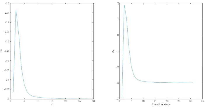
Example 5.1. LetH₌R, the set of all real numbers, with the inner product defined by_〈x,y_{〉 =} x y, _∀x,y_∈R, and induced usual norm_|._|. LetC₌[₋4, 2]; letF1,F2:C×C→Rbe defined by

F1(x,y)=(3−x2)(x−y),F2(x,y)=(x+6)(y−x), ∀x,y∈C; letψ1,ψ2:C→Hbe defined by

ψ1(x)₌2x,ψ2(x)₌x,_∀x_∈C and let for eachx_∈R, we definef(x)₌1₆x, A(x)₌1₃x, B(x)₌ 1

10x, and let, for eachx∈C,T(s)x=x. Then there exist unique sequences {xn}⊂R, {un,i}⊂C, and {wn}⊂Cgenerated by the iterative schemes

un,i=TrFni,i(xn−rn,iψixn), wn= 1

2(un,1+un,2) (5.1)

xn+1= 1

nxn+

1

10(n+1)2xn+ ³

(1₋ 2

n2)I− 1 (n+1)2B−

3

nA

´1

sn

Zsn

0

wnd s (5.2)

whereαn = _n3, βn = _(n+1₁₎2, ǫn =_n22 andsn =n, rn,1=rn,2=1+_n1. Then {xn} converges to

{−3}∈Tk

i₌1Fix(S)∩GEP(Fi,ψi).

Proof. The bifunctionsF1andF2satisfy the (A1)−(A4). Further, f is contraction mapping with constantα₌1₃andAandBare strongly positive bounded linear operator with constant

¯

δ₌1 onR. Therefore, we can chooseγ₌2 which satisfies 0<γ_<αδ¯_<γ_+α1. Furthermore, it is easy to observe thatTk

i₌1Fix(S)∩GEP(Fi,ψi)={−3}6= ;. We have computedun,i for each example i = 1,2 as follow

un,1= − 1₊

q

1₋4(1_+n1)((1_+n2)xn−3(1+_n1))

2+n2

,

un,2= − 1

nxn+6(1+

1

n)

2+n1

, wn=

1

2(un,1+un,2)

xn₊1=

³10n2+21n+10 10n(n₊1)2

´

xn+

³10n4+10n3−31n2−50n−20 10n2_(n+1)2

´

wn.

Figure 1: The graph of {xn} with initial valuex1=1.

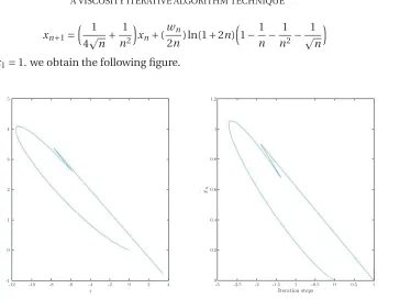
Example 5.2. Let H₌R, the set of all real numbers, with the inner product defined by_〈x,y_{〉 =} x y, ∀x,y∈R, and induced usual norm|.|. Let C=[0, 2]; let F1,F2,F3:C×C →Rbe defined

by F1(x,y)= −2x2(x₋y), F2(x,y)= −x2(x₋y)2, F3(x,y)= −3x2₊x y₊2y2, ∀x,y _∈C ; let ψ1,ψ2,ψ3:C →H be defined byψ1(x)=ψ2(x)=ψ3(x)=0, ∀x∈C and let for each x∈R,

we define f(x)₌ 1₈x, A(x)₌B(x)₌I , and let, for each x_∈C, T(s)x₌₁₊1_2sx. Then there exist unique sequences{xn}⊂R, {un,i}⊂C , and{wn}⊂C generated by the iterative schemes

un,i=TrFni,i(xn−rn,iψixn), wn= 1

3(un,1+un,2+un,3) (5.3)

xn₊1= 2 8pnxn+

1

n2xn+ ³

(1₋1

n)I−

1

n2B− 1

p nA

´ 1

sn

Zsn

0 1

1₊2swnd s (5.4) whereαn=p1_n, βn=_n12, ǫn=

1

n and sn=n,rn,1=rn,2=1+

8

n. Then{xn}converges to{0}∈

Tk

i₌1Fix(S)∩GEP(Fi,ψi).

Proof. It is easy to prove that the bifunctionsF1,F2andF3satisfy the (A1)−(A4). Further,

f is contraction mapping with constantα₌1₅ andA=B=I are strongly positive bounded linear operator with constant ¯δ₌1 on R. Therefore, we can chooseγ₌2 which satisfies 0<γ<δα¯<γ+

1

α. Furthermore, it is easy to observe that Tk

i=1Fix(S)∩GEP(Fi,ψi)={0}6= ;. We have computedun,ifor i = 1,2 as follow

un,1=

−1₊q1₊(8₊64_n)xn

4₊32_n , un,2=xn, un,3=

n

6n₊40xn

wn=

1

xn+1= ³ 1

4pn+

1

n2 ´

xn+( wn

2n) ln(1+2n)

³ 1−1

n−

1

n2− 1

p_n ´

Choosex1=1. we obtain the following figure.

Figure 2: The graph of {xn} with initial valuex1=1.

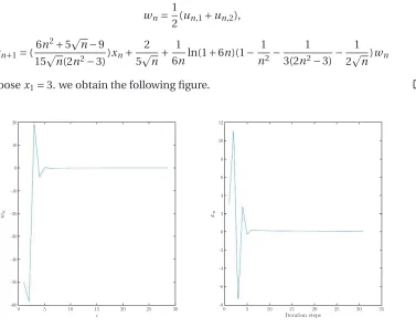
Example 5.3. Let H=R, the set of all real numbers, with the inner product defined by〈x,y〉 = x y, ∀x,y∈R, and induced usual norm|.|. Let C =[0, 3]; let F1,F2:C×C→Rbe defined by

F1(x,y)=5x(x−y), F2(x,y)= −2x(y−x), ∀x,y∈C ; letψ1,ψ2:C→H be defined byψ1(x)= 3x,ψ2(x)=4x,∀x∈C and let for each x∈R, we define f(x)= 1₅(x+2), A(x)=x, B(x)=1₃x,

and let, for each x_∈C, T(s)x₌₁₊1_3sx. Then there exist unique sequences{xn}⊂R, {un,i}⊂C , and{wn}⊂C generated by the iterative schemes

un,i=TrFni,i(xn−rn,iψixn), wn= 1

2(un,1+un,2) (5.5)

xn+1= 1

5pn(xn+2)+

1

3(2n2₋₃₎xn+ ³

(1₋ 1

n2)I− 1 2n2₋₃B−

1 2pnA

´1

sn

Zsn

0 1

1+3swnd s (5.6) whereαn=₂p1_n,βn=_2n12₋₃, ǫn=

1

n2 and sn=2n,rn,1=rn,2=1+

1

5n2. Then{xn}converges to

{0}∈Tk

i₌1Fix(S)∩GEP(Fi,ψi).

Proof. It is easy to prove that the f is contraction mapping with constantα₌1₃ andA and

B are strongly positive bounded linear operator with constant ¯δ₌1 on R. Therefore, we can chooseγ=2 which satisfies 0<γ< δα¯ <γ+

1

α. Furthermore, it is easy to observe that Tk

i₌1Fix(S)∩GEP(Fi,ψi)={0}6= ;. As mention

un,1=

10n2+3

50n2₊₅xn, un,2=

wn=

1

2(un,1+un,2),

xn₊1=(

6n2₊5pn₋9 15pn(2n2₋₃₎)xn+

2 5pn+

1

6nln(1+6n)(1−

1

n2−

1 3(2n2−3)−

1 2pn)wn

Choosex1=3. we obtain the following figure.

Figure 3: The graph of {xn} with initial valuex1=3.

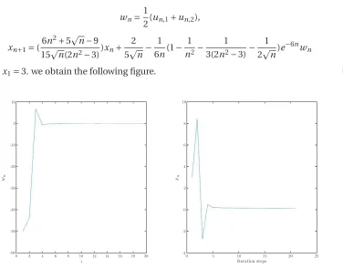
Example 5.4. Let H₌R, the set of all real numbers, with the inner product defined by_〈x,y_{〉 =} x y, _∀x,y_∈R, and induced usual norm_|._|. Let C ₌[0, 3]; let F1,F2:C×C→Rbe defined by

F1(x,y)=5x(x−y), F2(x,y)= −2x(y−x), ∀x,y∈C ; letψ1,ψ2:C→H be defined byψ1(x)= 3x,ψ2(x)₌4x,_∀x_∈C and let for each x_∈R, we define f(x)₌1₅(x₊2), A(x)₌x,B(x)₌1₃x, and let, for each x_∈C,T(s)x₌e−3s_{x. Then there exist unique sequences{x}

n}⊂R, {un,i}⊂C , and{wn}⊂C generated by the iterative schemes

un,i=TrFni,i(xn−rn,iψixn), wn= 1

2(un,1+un,2) (5.7)

xn₊1= 1

5pn(xn+2)+

1

3(2n2₋₃₎xn+ ³

(1₋ 1

n2)I− 1 2n2₋₃B−

1 2pnA

´ 1

sn

Zsn

0

e−3swnd s (5.8)

whereαn=₂p1_n, βn=_2n12₋₃,ǫn=_n12 and sn=2n,rn,1=rn,2=1+₅1_n2. Then{xn}converges to

{0}_∈Tk

i=1Fix(S)∩GEP(Fi,ψi).

Proof.By the same arguments example (5.3), we have

un,1=

10n2+3

50n2₊₅xn, un,2=

wn=

1

2(un,1+un,2),

xn+1=(

6n2₊5pn₋9 15pn(2n2₋₃₎)xn+

2 5pn−

1 6n(1−

1

n2− 1 3(2n2₋₃₎−

1 2pn)e

−6n_w n

Choosex1=3. we obtain the following figure.

Figure 4: The graph of {xn} with initial valuex1=3.

References

[1] E. Blum and W. Oettli,From optimization and variational inequalities to equilibrium problems, Math. Stud.,

63(1994), 123–145.

[2] S. S. Chang, J. Lee and H. W. Chan,An new method for solving equilibrium problem, fixed point problem and variational inequality problem with application to optimization, Nonlinear Analysis.,70(2009), 3307–3319. [3] F. Cianciaruso, G. Marino and L. Muglia,Iterative methods for equilibrium and fixed point problems for

non-expansive semigroups in Hilbert space, J. Optim. Theory Appl.,146(2010), 491–509.

[4] F. Cianciaruso, G. Marino, L. Muglia and Y. Yao,A hybrid projection algorithm for finding solution of mixed equilibrium problem and variational inequality problem, Fixed Point Theory Appl.,2010(2010), 383740. [5] P. L. Combettes and A. Hirstoaga,Equilibrium programming in Hilbert space, J. Nonlinear Convex Anal.,6

(2005), 117–136.

[6] J. Kang, Y. Su and X. Zhang,Genaral iterative algorithm for nonexpansive semigroups and variational in-equalitis in Hilbert space, Journal of Inequalities and Applications, (2010) Article ID.264052, 10 pages. [7] K. R. Kazmi and S. H. Rizvi,Iterative approximation of a common solution of a split general- ized equilibrium

problem and a fixed point problem for nonexpansive semigroup, Math. Sci.,7(2013), Art. 1.

[8] G. Marino and H. K. Xu,A general iterative method for nonexpansive mappings in Hilbert spaces, Math. Appl.,

318(2006), 43–52.

[9] A. Moudafi and M. Thera,Proximal and Dynamical Approaches to Equilibrium Problems, in: Lecture Notes in Economics and Mathematical Systems, vol.477, Springer, 1999, 187–201.

[11] N. Nadezhkina and W. Takahashi,Weak convergence theorem by an extragradient method for nonexpansive mapping and monotone mapping, J. Optim. Theory Appl., 128 (2006) 191–201.

[12] Z. Opial,Weak convergence of the sequence of successive approximations for nonexpansive mappings, Bull. Am. Math. Soc.,73(4)(1967), 595–597.

[13] S. Plubtieng and R. Punpaeng,Fixed point solutions of variational inequalities for nonexpansive semigroups in Hilbert spaces, Math. Comput. Model.,48(2008), 279–286.

[14] H. R. Sahebi and A. Razani,A solution of a general equilibrium problem, Acta Mathematica Scientia,33B(6) (2013), 1598–1614.

[15] H. R. Sahebi and A. Razani,An iterative algorithm for finding the solution of a general equilibrium problem system, Faculty of Sciences and Mathematics, University of Nis, Serbia,7(2014), 1393–1415.

[16] H. R. Sahebi and S. Ebrahimi,An explicit viscosity iterative algorithm for finding the solutions of a general equilibrium problem systems, Tamkang Journal Of Mathematics46(3)(2015), 193–216.

[17] H. R. Sahebi and S. Ebrahimi,A Viscosity iterative algorithm for the optimization problem system, Faculty of Sciences and Mathematics, University of Nis, Serbia,8(2017), 2249–2266.

[18] T. Shimizu and W. Takahashi,Strong convergence to common fixed points of families of nonexpansive map-pings, J. Math. Anal. Appl.,211(1997), 71–83.

[19] T. Suzuki,Strong convergence of Krasnoselskii and Mann’s type sequences for one parameter nonexpansive semigroups without Bochner integrals, J. Math. Anal. Appl.,305(2005), 227–239.

[20] M. Taherian and M. Azhini,Strong convergence theorems for fixed point problem of infinite family of non self mapping annd generalized equilibrium problems with perturbation in Hilbert spaces, Advances and Applica-tions in Mathematical Sciences,15(2) (2016), 25–51.

[21] W. Takahashi and M. Toyoda,Weak convergence theorems for nonexpansive mappings and monotone map-pings,118(2003), 417–428.

[22] S. Takahashi and W. Takahashi,Viscosity approximation method for equilibrium and fixed point problems in Hilbert space, J. Math. Anall. Appl.,331(2007), 506–515.

[23] S. Takahashi and W. Takahashi,Strong convergence theorem for a generalized equilibrium problem and a nonexpansive mapping in a Hilbert space, Nonlinear Anal.,69(2008), 1025–1033.

[24] H. H. Xu and T.H. Kim,Convergence of hybrid steepest-descent methods for variational inequalites, J. Optim. theory Appl.,119(2003), 185–201.

[25] H. K. Xu,Viscosity approximation method for nonexpansive semigroups, J. Math. Anal. Appl.,298(2004), 279– 291.

[26] Y. Yao, J. C. Yao,On modified iterative method for nonexpansive mappings and monotone mappings, Appl. Math. Comput.,186(2007), 1551–1558.

[27] L. C. Zeng and Y. Yao,Strong convergence theorem by an extragradient method for fixed point problems and variational inequality problems, Taiwanese J. Math.,10(2006), 1293–1303.

Department of Mathematics, Science and Research Branch, Islamic Azad university, Tehran, Iran.

E-mail:[email protected]

Department of Mathematics, Science and Research Branch, Islamic Azad university, Tehran, Iran.

E-mail:[email protected]

Department of Mathematics, Ashtian Branch, Islamic Azad university, Ashtian, Iran.