Paper 15-2007

A comparative Study of Contact Problems Solution Based on the Penalty

and Lagrange Multiplier Approaches

S. Vulovic, M. Zivkovic, N. Grujovic, R. Slavkovic

Faculty of Mechanical Engineering

University of Kragujevac, S. Janjic 6, 34000 Kragujevac, Serbia e-mail: [email protected]

Abstract

Numerical models based on the penalty and Lagrange multiplier method for contact problems with friction are compared in this paper. The presented approaches, with use of Coulomb’s frictional law, elasto-plastic tangential slip decomposition, and consistent linearization, result in quadratic rates of convergence with the Newton-Raphson iteration. A standard contact search algorithm independent of the formulation is used for the detection of contact between previously separate meshes and for the application of displacement constraints where contact was identified.

The models have been implemented into a version of the computational finite element program PAK [3]. Numerical examples that illustrate performance of the described procedures are given.

Key words: contact problem, penalty method, Lagrange method, Coulomb’s law

1. Introduction

Contact mechanics has its application in many engineering problems. The interaction between soil and foundations in civil engineering, general bearing problems as well as bolt and screw joints in mechanical engineering, are examples of small deformation contact problems. On contrary, the impact of cars, car tire-road interaction and metal forming are large deformation contact problems. Here, nonlinear material laws, damage, dynamic fatigue, friction, wear, etc. must be taken into account to design optimal components and assemblies.

Effective application of finite element contact solvers demands a high degree of experience since the general robustness and stability cannot be guaranteed. For this reason the development of more efficient, fast and stabile finite element contact discretizations is still a hot topic, especially due to the fact that engineering applications become more and more complex.

2. Formulation of the multi-body frictional contact problem

A contact between two deformable bodies is considered. As the configuration of two bodies coming into the contact is not a priori known, the contact represents a nonlinear problem even when the continuum behaves as a linear elastic material.

2.1 Contact kinematics

Two bodies are considered: _B(1) _{and B}(2)_{, Fig. 1. We will denote the contact surface} ( )i C

Γ as the part of the body _B(i) _{such that all material points where contact may occur at any time t are}

included.

Using a standard notation in contact mechanics we will assign to each pair of contact surfaces involved in the problem as slave and master surfaces. In particular, let (1)

C

Γ is taken to be the slave surface and (2)

C

Γ is the master surface. The condition which must be satisfied is that any slave particle cannot penetrate the master surface.

Let x be the projection point of the current position of the slave node _xk _{onto current} position of the master surface (2)

C

Γ , defined as

1 2

1 2 1 2

( , )

( , ) 0 ( , )

k

k α

ξ ξ _{ξ ξ} ξ ξ

−

⋅ =

−

x x

a

x x (1)

where 1, 2α = and _{( ,}1 2₎

α ξ ξ

a are the tangent covariant base vectors at the point.

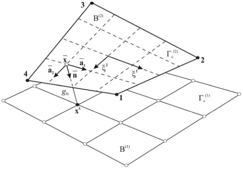
The definition of the projection point allows us to define the distance between any slave node and the master surface. The normal gap or the penetration gN for slave node k is defined as the distance between current positions of this node with respect to the master surface (2)

C Γ

( k ) N

g = x − ⋅x n (2)

where n refers to the normal to the master face (2)

C

Γ at point x (Fig. 1). Normal to be defined using tangent vectors at the point x is

1 2

1 2

× =

× a a n

Fig. 1. Geometry of a 3D node-to-segment contact element.

This gap (2) gives the non-penetration conditions as follows:

0 perfect contact; 0 no contact; 0 penetration

N N N

g = g > g < (4)

If the analyzed problem is frictionless, the function (4) completely defines the contact kinematics. However, if the friction is modeled, tangential relative displacement must be introduced. In this case the sliding path of the node _xk _{over the contact surface} (2)

C Γ is described by total tangential relative displacement as

0 0 0

t t t

T T

t t t

g =

∫

∫

∫

within a time interval from t0 to t.

The time derivatives of parameter ξα in equation (6) can be computed from the relation (1), [8]. In the geometrically linear case we obtain the following result:

k

T

aβαξ&β =⎡⎣x& −x a&⎤⎦⋅ α =g& α (6)

where aαβ =a aα⋅ β is the metric tensor at point x of the master surface Γ(2)C . From the equations (5) and (6) we can deduce the relative tangential velocity at the contact point

T gT

α α

α α

ξ

= =

g& & a & a (7)

2.2 Constitutive equations for contact interface

For mathematical and computational modeling the surface characteristics have to be put into the constitutive interface constraint.

A contact stress vector t with respect to the current contact interface (2)

C

Γ can be split into a normal and tangential parts,

N T tN tT

α α

= + = +

zero in the case of frictionless contact. When the contact occurs, one has the condition t_N <0. If there is no penetration between the bodies, then the relations g_N >0 and t_N =0 hold. This leads to the statements

0, 0, 0

N N N N

g ≥ t ≤ t g = (9)

which are known as Kuhn-Tucker conditions.

In the tangential direction a distinction is made between stick and slip. As long as no sliding between to bodies occurs, the tangential relative velocity is equal to zero. If the velocity is zero, also the tangential relative displacement (5) is zero. This state is called the stick case with the following restriction:

T = ⇔ T =

g& 0 g 0 (10)

A relative movement between two bodies occurs if the static friction resistance is overcome and the loading is large enough such that the sliding process can be kept. Therefore, the relative sliding velocity, with respect to the sliding displacement, is in the opposite direction to the friction force. With this, the tangential stress vector is restricted as follows:

sl

sl T

T N _sl

T

g

t α

α = −μt

g

&

& (11)

where μ is the friction coefficient. In the simplest form of Coulomb’s law (11), μ is constant and no distinction is made between static and sliding friction.

After the introduction of the stick and slip constraints, one needs an indicator to decide whether stick or slip actually takes place. Therefore, an indicator function

-T N

f = t μt (12)

is evaluated, which respect to the Coulomb’s model for frictional interface law. In equation (12) the first term is _T = t a t_T αβ_T

α β

t . Then the following contact states can be distinguished:

- 0 Stick - >0 Slip

T N

T N

t f

t

μ μ

⎧ ≤ →

⎪

= ⎨ _→

⎪⎩ t

t (13)

Using the penalty method for normal stress, the constitutive equation can be formulated as

N N N

t =ε g (14)

where εN is the normal penalty parameter. The tangential part is different for the stick and for the slip cases. For the stick, a simple linear constitutive model can be used to describe the tangential stress

stick

T T T

tα =ε gα (15)

assumed, the trial values of the tangential contact pressure vector tTα, and the indicator function f at load step n+1 can be expressed in terms of their values at load step n, as follows

1 1 1

trial

T n T n T T n T n T n

t t g t a β

α + = α + Δε α + = α +ε αβΔξ + (16)

1 1 1

trial trial

Tn Tn Nn

f ₊ = t ₊ −μt ₊ (17)

The return mapping is completed by

1 1

1 1

if 0

if 0 trial

T n

T n trial

Nn T n

f t t f t n α α α μ + + + + ⎧ ≤ ⎪

= ⎨ _>

⎪⎩ (18)

with

1 1

1

trial

trial T n

T n trial

Tn t n α α + + + =

t (19)

The penalty method can be illustrated as a group of linear elastic springs that force the body back to the contact surface when overlapping or sliding occurs.

2.3 Equilibrium equation for bodies in contact

When two bodies at time t are in contact, the principle of virtual work can be written as (for a detailed legend of the symbols see [8])

(

)

2

1

: _c 0

V V _S

grad dV dV dA C

α α α σ α α α α α α α α α δ ρ δ δ = ⎛ ⎞ ⎜ _{− − − ⋅ ⋅} ⎟_{− =} ⎜ ⎟ ⎝ ⎠

∑ ∫

∫

∫

( ) ( ) ( )

( ) ( ) ( ) ( ) _&&( ) ( ) ( ) ( ) ₍₂₀₎

where C_c is “contact contribution”. For the Lagrange multiplier method for contact with friction, the contact contribution are formulated for stick as

(

)

C

c N N T T

S

C =

_∫

and for case of sliding it is

(

)

C

c N N T T

S

C =

_∫

where δg_N and δg_T are the variations of gap and tangential displacement; λ_N and λ_T are normal and tangential Lagrange multipliers and tT is tangential stress vector which is determined from the constitutive law for frictional slip. Note that the Lagrange multiplier λ_N can be identified as the contact stress tN.

Contact contribution for the penalty method are formulated as follow

(

)

C

c N N N T T

S

The virtual work of boundary nodes which are in contact is formulated for a slave node k:

k T

c N N T T N k N T k T N k N T k c c

C =F gδ +F gδ =t A gδ +t Aδg =t A gδ +t Aα δξα =δu F (24)

Here, the quantities are: F_N =t A_{N k} the normal force; F_Tα =t A_Tα _k the tangential force [8]; Ak the area of the contact element; F_c the contact force vector.

For the penalty method we define a displacement vector for the five-node contact elements (k, 1, 2, 3, 4)

{

}

T k

c

δu = δu δu δu δu δu (25)

and the vectors

1 2 3 4 H H H H ⎧ ⎫ ⎪₋ ⎪ ⎪ ⎪ ⎪ ⎪ = −_{⎨ ⎬} ⎪₋ ⎪ ⎪ ⎪ − ⎪ ⎪ ⎩ ⎭ n n N n n n 1 2 3 4 H H H H β β β β β β ⎧ ⎫ ⎪₋ ⎪ ⎪ ⎪ ⎪₋ ⎪ = ⎨ ⎬ ⎪₋ ⎪ ⎪ ⎪ − ⎪ ⎪ ⎩ ⎭ a a a T a a

Dα =aαβTβ (26)

Thus, the contact force vector can be expressed by (26) for the slave node k which is in contact, by

c FN FT

α α

⎡ ⎤

=_⎣ + _⎦

F N D (27)

The contact forces FN and FTα in (27) can be obtained by multiplying the constitutive

interfaces laws (15), (16) and (18) by the area of the contact element A_k.

3.3 Algorithm for frictional contact

In order to apply Newton’s method for the solution of nonlinear system of the equilibrium equation (20), a linearization of the contact contributions is necessary. The linearization of the equation (25), for the infinitesimal theory, gives

T

N N T c c c

t g t α

α

δ δξ δ

Δ + Δ ⋅ = u K uΔ (28)

where K_c is the contact stiffness matrix of contact element. It is assumed that the contact area

k

A is not changing significantly so the area Ak is contained within the penalty parameters. The tangent stiffness matrix for the normal contact is

T

N =εN

K NN (29)

Analogous to (29) we obtain the symmetric tangent stiffness matrix for stick condition,

stick T

T Ta

α β αβ

ε

=

K D D (30)

1

1 1 1

1

slip trial T N Nn trial trial T

T N T n trial T T n T n

Tn

g

n α a β n n β α γ

α βγ α α

με

με + ε δ

+ + +

+

⎡ ⎤

= + _⎣ − _⎦

K D N D D

t (31)

The second term in the tangent matrix is non-symmetric. This is because the Coulomb’s of friction can be viewed as a non-associative constitutive equation.

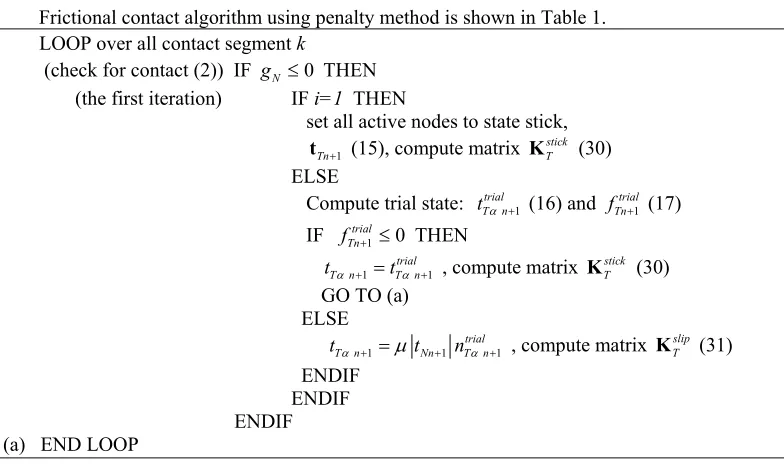
Frictional contact algorithm using penalty method is shown in Table 1. LOOP over all contact segment k

(check for contact (2)) IF g_N ≤0 THEN (the first iteration) IF i=1 THEN

set all active nodes to state stick, t_Tn+1 (15), compute matrix stick

T K (30) ELSE

Compute trial state: tTtrialαn+1 (16) and fTntrial+1 (17)

IF fTntrial+1 ≤0 THEN

tTαn+1=tTtrialαn+1 , compute matrix KTstick (30) GO TO (a)

ELSE

_{1 1} trial ₁

T n Nn T n

t α + =μt + nα + , compute matrix KslipT (31) ENDIF

ENDIF ENDIF (a) END LOOP

Table 1. Frictional contact algorithm using the penalty method

The linearization of the equations (21) and (22) gives the stiffness matrix for Lagrange multiplier method

T

N N T c c

t δg tα δξα δ λ

Δ + Δ ⋅ = u K Δu (32)

Detailed description of the Lagrange multiplier method contact stiffness matrix is given in reference [1].

Finally, we obtain the global nonlinear finite element equation for the penalty method as

[

]

+ + = −

MU&& K K U F F (33)

and for Lagrange multiplier method ,

0 0 0 ( )

0 0 0 0 0 0 N

t g

λ λ

λ

⎧⎡ ⎤ ⎡ ⎤ ⎡ ⎤ Δ⎫⎡ ⎤ ⎡ ⎤ ⎡ ⎤

⎪ _{+ +} ⎪ _{= −}

⎨⎢ ⎥ ⎢ ⎥ ⎢ ⎥⎬⎢_Δ ⎥ ⎢ ⎥ ⎢ ⎥

⎣ ⎦ ⎣ ⎦ ⎣ ⎦ ⎣ ⎦

⎪ ⎣ ⎦⎪ ⎣ ⎦

⎩ ⎭

M K K U F F

λ

K n (34)

where: Mis mass matrix; K is stiffness matrix and vector ( )Ft corresponds to an external force. The contact force vector for the 3D contact elements for the Lagrange multiplier method is

[

]

T _{H H H H}

λ =

Compression of a cylinder between two parallel plates is considered. Initial dimensions of the cylinder are: radiusr=6.35mm, height h=2r. Elasto-plastic material model with following yield curve is used

(

)

(

)

0 0 1 p

e

y y y y e H ep

δ

σ σ σ σ − δ

∞

= + − − + (36)

Material constants are: E=210.40 GPa, ν =0.3118, K=164.206 GPa, G=80.1938 GPa,

0 0.45 GPa

y

σ = , σ_y∞ =0.75 GPa, δ =16.96 GPa, H=0.12924 GPa. Due to symmetry, one-eight of the cylinder is modeled, with symmetry conditions for nodes lying in coordinate planes. It is assumed that there is no friction, and the solutions are obtained using contact element based on the Lagrange multiplier (see [1]) and penalty methods.

0 200 400 600 800 1000

0.0 0.5 1.0 1.5 2.0 2.5 3.0 3.5 4.0 4.5 5.0

Displacement [mm]

For

ce

[

kN

]

Lagrange 10E 100E 1000E

Fig. 2. Force – displacement relationship.

Deformation of the cylinder is increased by prescribed displacement at the plate. Solution is obtained by 25 steps of displacement increments equal to 0.2 mm; and by full-Newton iteration method with line search. The three different values for normal penalty parameter are considered: a) ε = ⋅_N 10 E; b) ε =_N 100⋅E and c) ε =_N 1000⋅E. The force - displacement diagram is shown in Fig. 2. In this example, a penalty number which is chosen have to be at least 100 times larger then E, for good approximation of the normal force. It is obvious that the value of the penalty parameter has the effect on accuracy of the results in contact problems. Initial and deformed configurations at the final step are shown in Fig. 3.

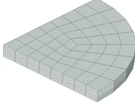
4.2 The contact between an elastic ring and a foundation

An elastic ring consists of an outer and inner rings of the same thickness t=5 UL with different materials. The geometry and material parameters are given in Fig. 4. A total downward displacement of u=40 UL is applied to the ring at its top end in 80 steps. The computation is performed for both Lagrange and penalty formulations ( 5

N 10 UL

ε = ).

Fig. 4. The elastic ring with the foundation.

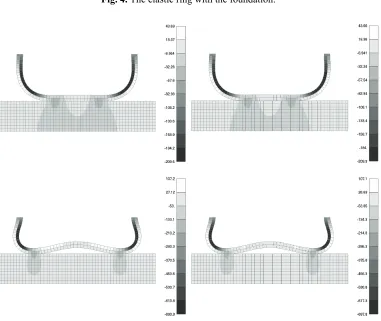
Fig. 5. Vertical stress field and deformation configuration, left panel: the Lagrange multiplier formulation; right panel: the penalty formulation

(upper figures – step 44; lower figures – step 80).

Inner ring: E=105 _UF/UL2 ν=0.3

Outer ring: E=103 _UF/UL2 ν=0.3

are shown in Fig. 5, for step 44 step 80.

5. Conclusions

In the paper a model for three-dimensional contact problem with friction based on the penalty and Lagrange multiplier method was described. Due to the intrinsic similarity between friction and the classical elasto-plasticity [9,10], the constitutive model for friction can be constructed following the same formalism as in classical elasto-plasticity. Using the penalty method, the computation time is smaller but the results are strongly dependent on the value of the penalty factor. The Lagrange multiplier method leads to exact solution but with more iterations and significant increase of the number of degrees of freedom, i.e. equations, and thus reduces computational efficiency. The numerical examples indicate a possibility of easy comparative simultaneous use of both procedures in the analysis of finite deformation problems within the same computer code.

References

[1] Grujovic N., Numerical solution of contact problems, Monograph, Faculty of Mech. Eng. Univ. of Kragujevac, Kragujevac, 2005.

[2] Slavkovic R., M. Zivkovic, M. Kojic, N. Grujovic, Large strain elastoplastic analysis using incompatible displacements, in: XXII Yugoslavian congress of the theoretical and applied mechanics, June 2-7, Vrnjacka banja, 1997.

[3] Kojic M., R. Slavkovic, M. Zivkovic, N. Grujovic, The software packages PAK, Faculty of Mechanical Engineering of Kragujevac, Serbia and Montenegro.

[4] Fisher K.A., Mortal type methods applied to nonlinear contact mechanics, Ph.D. Thesis, Institut für Bumechanick und Numerische Mechanik Univ. of Hannover, Hannover, 2005.

[5] Laursen T.A., J.C. Simo, A continuum-based finite element formulation for the implicit solution of multibody, large deformation frictional contact problems, Inter. J. Num. Meth. Eng. 36 3451-3485, 1993.

[6] Peric Đ., R.J. Owen, Computational model for 3-D contact problems with friction based on the penalty method, Inter. J. Num. Meth. Eng. 35 1289-1309, 1992.

[7] Wriggers P., T.V. Van, E. Stein, Finite element formulation of large deformation impact-contact problems with friction, Computers and Structures. 37 319-333, 1990. [8] Wriggers P., Computational Contact Mechanics, J. Wiley & Sons Ltd, West Sussex,

England, 2002.

[9] Kojic M., K. J. Bathe, Inelastic Analysis of Solids and Structures, Springer, Berlin-Heidelberg, 2005.