Simultaneous Optimization of Quantitative and Ordinal
Responses Using Taguchi Method
S. Pal1, S. Gauri2
1Statistical Quality Control and Operations Research Unit, Indian Statistical Institute, 110, Nelson Manickam Road, Chennai- 600029, India.
2Statistical Quality Control and Operations Research Unit, Indian Statistical Institute, 203 B. T. Road, Kolkata-700108, India.
A B S T R A C T
In the real world, the overall quality of a product is often represented partly by the measured values of some quantitative variables and partly by the observed values of some ordinal variables. The settings for the manufacturing processes of such products are required to be optimized considering the quantitative as well as the ordinal response variables. But the simultaneous optimization of the quantitative and the ordinal response variables are rarely attempted by the researchers. In this paper, a new approach for simultaneous optimization of quantitative and ordinal responses are presented, which are developed by integrating multiple regression techniques, ordinal logistic regression technique, and Taguchi’s Signal-to-Noise Ratio (SNR) concept. The effectiveness of the proposed method is evaluated by analyzing two experimental data sets taken from the literature. The comparison of results reveals that the proposed method leads to the best optimal solution with respect to the total SNR as well as the Mean Square Error (MSE) of individual responses.
Keywords: Quantitative responses, Ordinal responses, Multiple regression, Ordinal logistic regression, Taguchi method, Optimization.
Article history: Received: 20 March 2018 Revised: 09 June 2018 Accepted: 10 August 2018
1. Introduction
For survival in today’s highly competitive world, it is essential for a manufacturing organization
to produce the high quality product consistently, and one of the basic requirements towards achieving this goal is to use the optimal process setting at every stage of the manufacturing operations. Over the years, Taguchi’s robust design method [1] has gained the maximum popularity among the engineers for accomplishing the task of optimization of process parameters. Taguchi [1] applied the quality loss function to evaluate the product quality and employed Signal-to-Noise Ratio (SNR) with simultaneous consideration of achieving the target and reducing the
Corresponding author
Email: [email protected] DOI: 10.22105/riej.2018.127858.1039
International Journal of Research in Industrial
Engineering
variability around the target value of the response variable. However, Taguchi [1] focused on optimization of a single quality characteristic only; whereas most of the modern manufacturing processes usually have several response variables. Therefore, many researchers were motivated to develop the appropriate methodologies for multi-response optimization. A branch of research has been directed towards developing the methodologies using the classical statistical techniques like response surface methodology and optimization search algorithms [2-7]. But, these approaches are mathematically rigorous and consequently are not easy to implement in industries. Several other researchers have taken interest in developing appropriate methodologies for optimizing multiple responses under Taguchi’s robust design framework [8-12]. However, all these researchers make an implicit assumption that all the responses are quantitative variables, and thus, their proposed methodologies for multi-response optimization are applicable only if all the response variables are quantitative in nature.
However, in real world, the complete quality of a product is often represented partly by measured values of some quantitative response variables and partly by the measured (judged) values of some ordinal response variables. In such cases, the analysis of quantitative response variables and ordinal response variables separately usually are not much useful. This is because the optimal parametric settings with respect to the quantitative response variables and the ordinal response
variables are different. For resolving the conflict in the optimal factor levels, the process engineer
is required to use his/her relevant experience and engineering knowledge, implying that the uncertainty in the optimal factor levels will be increased.
An appropriate methodology which is capable of optimizing simultaneously the quantitative as
well as ordinal variables can truly satisfy the practical need of the industries. It is observed from the extensive survey of literature that only Wu [17] and Hsieh and Tong [29] have attempted to optimize the quantitative and ordinal response variables simultaneously under Taguchi’s framework of robust design approach. Wu [17] treated the ordinal data as continuous variable. Assuming the lower bound of a defined category as the weight for that category, he computed the weighted average quality loss for the ordinal data. Then, he computed total quality loss for all response variables and transformed it to SNR, which is maximized to derive the optimal process settings. On the other hand, Hsieh and Tong [29] applied artificial neural networks for simultaneous optimization of the quantitative and ordinal responses. The problem with Wu’s [17] approach is that it does not lead to efficient optimal solution. On the other hand, Hsieh and Tong’s artificial intelligence–based techniques [29] does not help engineers to learn efficient engineering experiences during the period of the optimizing process. Also, it is quite difficult to be employed in industries. In this article, a new procedure for simultaneous optimization of quantitative and ordinal response variables is proposed, which results in superior optimization performance with respect to total SNR and MSE of individual response variables. In the proposed method, a new performance metric is defined that integrates logistic regression technique, multiple regression technique and Taguchi’s SNR concept. The process parameter is optimized by maximizing the developed performance metric.
This article is organized as follows. Section 2 describes the framework of the proposed method for simultaneous optimization of the quantitative and ordinal response variables. The necessary steps for implementing of the proposed method are summarized in Section 3. Analysis of two sets of the past experimental data and related results are presented in Section 4. The future scope and the limitations of the present research are discussed in Section 5. The article is concluded in Section 6.
2. The Framework of the Proposed Method
means and the variances of the response variables based on the appropriately fitted multiple regression equations and then to compute SNRs using the predicted values instead of the observed values. It is well established that the probabilities in each category of the ordinal variable can be predicted by using the ordinal logistic regression model [18]. Jeng and Guo [25] showed that the MSE value can be computed from the predicted probabilities of the ordinal response variable and then, MSE value can be transformed into SNR value. Therefore, it is believed that the concept of MRWSN method can easily be extended in the cases where the simultaneous optimization of quantitative and ordinal response variables are required.
Suppose, the settings of m control factors (𝑥1, 𝑥2, … , 𝑥𝑚) are required to be optimized with respect to r continuous response variables and s ordinal response variables (each ordinal response have k levels or categories). Suppose, for the purpose of optimizing the process settings, an orthogonal experimentation with n trial runs is designed and each trial run is replicated q times. In each replication, values of all the response variables are observed. Optimization such a process using the proposed method would require (i) fitting appropriate multiple regression equations for the means and variances of the quantitative responses, (ii) fitting appropriate ordinal logistic regression equations for the ordinal responses, (iii) computation of SNR values from the predicted means, variances, and cumulative probabilities, (iv) obtaining overall performance index and (v) optimizing the overall performance index.
2.1 Fitting Regression Equations for Means and Variances of the Quantitative Responses
In an experimentation set up, the different levels of the control factors in a trial run are represented by the numerical values like 1, 2, 3, etc. (i.e. each trial run has different set of level values of the input variables (control factors) X. On the other hand, the actual mean and the variance of each quantitative response variable in each trial can be obtained from the q replications. Thus, using these set of level values of the input variable X, the computed means and the variances corresponding to n trial runs, the appropriate multiple regression equations for predicting the means, and the variances of different quantitative response variables can be established easily.
The multiple regression models for mean and variance of ith quantitative response variable (Yi) (i= 1, 2, 3,...,r) are given in Eqs. (1) and (2), respectively. Here, the logarithm transformation of variance is used to ensure positive value of the variance at any combination of the input variables.
𝜇𝑦𝑖= 𝜃0+ 𝜃1𝑥1+ 𝜃2𝑥2+ ⋯ + 𝜃𝑚𝑥𝑚+ 𝜃𝑚+1̅̅̅̅̅̅̅𝑥1
2+ ⋯ + 𝜃
𝑝1𝑥𝑚−1𝑥𝑚+ 𝜀1, (1)
log(𝜎𝑦𝑖
2) = 𝛿
0+ 𝛿1𝑥1+ 𝛿2𝑥2+ ⋯ + 𝛿𝑚𝑥𝑚+ 𝛿̅̅̅̅̅̅̅𝑚+1𝑥12+ ⋯ + 𝛿𝑝2𝑥𝑚−1𝑥𝑚+ 𝜀2, (2)
where i’s and i’s are regression coefficients, m is the number of input variables (control
factors), 𝑝1 and 𝑝2 are the total number of regressor terms in respective equations and 𝜀1 and 𝜀2
with mean value as zero and with constant variance 𝜎𝑒2. It is important to note that the regression equations of mean and variance for a quantitative response may not include the same terms as regression variables. There may be some square terms or cross terms which may appear in the regression equation for mean but may not appear in the regression equation for variance and vice versa. But, the number of regression terms in any equation should be smaller than the number of trial runs in the designed experiment.
The regression coefficients of these regression models can be obtained by the least square method. The option of performing multiple linear regression analysis is available in Microsoft Excel and in many statistical software packages, e.g. MINITAB and STATISTICA. Using these packages, the appropriate multiple regression equations can be established; however, diagnostic checks must be performed for validating each fitted regression equations. The adequacy of fitted model can be checked using ANOVA and an F-test for significance of regression. Any kind of the possible anomalies can be detected by examining residual analysis in terms of various plots, e.g. normality plot of residuals, plot of residual versus individual regression variable, etc. If after the diagnostic checks no serious violations of model assumptions are detected, then the regression equations are assumed to be adequate to predict means and variances of the response variable.
2.2 Fitting Ordinal Logistic Regression Equations for Ordinal Responses
Let us assume that an ordinal response variable Y has k number of the ordered categories denoted by 1, 2, …, k, where k ≥ 3 and is integer. The number of observations (frequencies) in each category in an experimental run can be obtained from q number of the repeated samples corresponding to the experimental run. These frequencies can easily be converted into the individual and the cumulative probabilities for each k categories. Using the ordinal logistic regression, these cumulative probabilities are modeled as a function of input variables (control factors). Generally, a logit transformation of the cumulative probabilities are used as a link function while model the cumulative probabilities as a function of input variables and accordingly; this type of ordinal logistic regression models are named as cumulative logit models. If there are k categories for an ordinal variable (Y), then there will be k-1 cumulative logit models for describing first k-1 cumulative probabilities of Y. The cumulative probability for the last kth category is always equal to 1.
Let pi denotes the probability that the 𝑢𝑡ℎsample of the ordinal response variable Y falls in 𝑖𝑡ℎ category, that is𝑝𝑖= 𝑃(𝑦𝑢 = 𝑖), where 𝑖 = 1,2, … , 𝑘 and𝑢 = 1,2, … , 𝑞. The transformation
𝑙𝑜𝑔𝑖𝑡[𝑝𝑖] = ln ( 𝑝𝑖
1−𝑝𝑖)is called the logit transformation of probability 𝑝𝑖. Logit of the cumulative probability up to 𝑖𝑡ℎ category is defined as
𝑙𝑜𝑔𝑖𝑡[𝑃(𝑦𝑢≤ 𝑖)] = 𝑙𝑛
𝑃(𝑦𝑢 ≤ 𝑖)
1 − 𝑃(𝑦𝑢≤ 𝑖)
These 𝑙𝑜𝑔𝑖𝑡𝑠 of cumulative probabilities are modeled as the function of m input variables (control factors) 𝑥1, 𝑥2, … , 𝑥𝑚as shown below:
𝑙𝑜𝑔𝑖𝑡[𝑃(𝑦𝑢≤ 𝑖)] = 𝛼𝑖+ 𝛽1𝑥1+ 𝛽2𝑥2+ ⋯ + 𝛽𝑚𝑥𝑚, 𝑖 = 1,2, … , 𝑘 − 1; 𝑢 = 1,2, … , 𝑞 (4) The effect of input variables will be the same in all cumulative 𝑙𝑜𝑔𝑖𝑡 models for different categories of the ordinal variable Y that means the values of 𝛽𝑗 coefficients (𝑗 = 1,2, … , 𝑘 − 1) are the same in all𝑘 − 1 logit models. The only difference in these models is in the intercepts, i.e. 𝛼𝑖values. The {𝛼𝑖: 𝑖 = 1,2, … , 𝑘 − 1} is increasing in 𝑖 because the cumulative probability
𝑃(𝑦 ≤ 𝑖) increases in 𝑖 and the logit transformation is an increasing function of this cumulative probability.
From the cumulative logit models, the cumulative probabilities of ith category of the ordinal variable Y can be computed as
𝑃(𝑦 ≤ 𝑖) = exp (𝛼𝑖+ ∑ 𝛽𝑗𝑥𝑗
𝑚 𝑗=1 )
1 + exp (𝛼𝑖+ ∑𝑚𝑗=1𝛽𝑗𝑥𝑗
, 𝑖 = 1,2, … , 𝑘 − 1 (5)
From the cumulative probabilities of first k-1 categories, the individual probabilities of each of the k categories can be obtained. The individual probability of ith(i = 1, 2, ..., k) category can be computed using Eq. (6). By multiplying the individual probabilities for different categories by the sample size q, the expected frequencies in each of the k categories of the ordinal response variable can be obtained. The regression coefficients of the ordinal logistic regression models can be obtained by using any statistical package, e.g. Minitab, SPSS, etc. However, the usual goodness-of-fit tests and the diagnostic checks must be performed for validating the cumulative logit models for the ordinal data.
1 1 1 1 1 1 1 1 1 1 1 1 1 1 exp( )
, for 1
1 exp( )
exp( ) exp( )
( ) , 2, 3,..., 1
1 exp( ) 1 exp( )
exp( )
1 f
1 exp( )
m j j j m j j j m m
i j j i j j
j j
m m
i j j i j j
j j
m
k j j
j m
k j j
j x
i x
x x
P y i i k
x x x x
or i k.
2.3 The Signal-to-Noise Ratio (SNR)
2.3.1 SNR for quantitative response variables
Taguchi’s robust design method aims at achieving a target value of the response quality characteristic and minimizing variability around the target value. Accordingly, Taguchi [1] proposes to consider SNR as the measure of performance. The most notable aspect of SNR is that it combines the location and the dispersion of a quantitative response variable in a single performance measure. Taguchi [1] has defined different SNRs for different types of quantitative quality characteristics as follows:
For Smaller-the-Better (STB) type of characteristic,
𝑆𝑁𝑅 = −10𝑙𝑜𝑔10(
1 𝑛∑ 𝑦𝑖
2 𝑛
𝑖=1
(7)
For Larger-The-Better type (LTB) of characteristic,
𝑆𝑁𝑅 = −10𝑙𝑜𝑔10(
1 𝑛∑
1 𝑦𝑖2
𝑛
𝑖=1
(8)
For Nominal-The-Best (NTB) type of characteristic,
𝑆𝑁𝑅 = 10𝑙𝑜𝑔10(
𝜇𝑦2
𝜎𝑦2
),
(9) where y and y are the mean and standard deviation of the response variable Y.
The SNRs are always expressed in decibels irrespective of the measurement units of the quality characteristics, and according to the Taguchi philosophy the higher SNR values are desirable irrespective of the type of the quality characteristics.
On the other hand, statistically, an appropriate performance measure for a NTB type quantitative response variable can be the Mean Square Error (MSE) value [30] and it is expressed as follows:
𝑀𝑆𝐸 =1
𝑛∑ (𝑦𝑖− 𝑇) 2
𝑖 = (𝜇𝑦− 𝑇)2+ 𝜎𝑦2,
(10)
where T is the specified target for the response variable Y and n is the number of observations. It may be noted that the MSE function combines the location and the dispersion effects of the response variable. If the expected value of the response variable is very close to its target value with reasonably low variability, the MSE value for the variable will be quite small. So, minimization of the expected MSE is in agreement with the Taguchi’s robust design philosophy
2.3.2 SNR for ordinal response variables
Jeng and Guo [25] proposed a Weighted Probability Scoring Scheme (WPSS) for computing the location and the dispersion effects in case of an ordinal response variable. In this method, the categorical data is listed first in a progressively undesirable order and then, the more desirable category is given more weighted to make the location effect as the Larger-the-Better (LTB) type quantitative response variable. Let, there are K categories of an ordinal quality characteristic with first category representing the best quality and a weight WK = K – (k – 1), k = 1, 2, ..., K is assigned to each category. The location score W and the dispersion score d2 for a particular setting combination is then defined as
𝑊 = ∑ 𝑤𝑘𝑝𝑘 𝐾
𝑘=1
(11)
𝑑2= ∑[𝑤𝑘𝑝𝑘− (𝑇𝑎𝑟𝑔𝑒𝑡 𝑣𝑎𝑙𝑢𝑒)𝑘]2 𝐾
𝑘=1
, (12)
where𝑝𝑘is the proportion of observation in 𝑘𝑡ℎ category, and the target values are defined as
[𝐾, 0,0, … , 0] for Categories 1, 2,…, 𝐾, respectively.
As it can be observed from Eq. (10), the location and the dispersion effects can be combined in the MSE function; therefore, Jeng and Guo [25] have recommended to consider the MSE value as the performance measure for the ordinal response variable. By considering the location scores as LTB type of the quantitative characteristic, they derived that the approximated expected value is
𝐸[𝑀𝑆𝐸] ≅ 1 𝑊2(1 +
3𝑑2
𝑊2). (13)
This MSE measure can then be transformed into the SNR by the following equation:
𝑆𝑁𝑅 = −10𝑙𝑜𝑔10(𝑀𝑆𝐸) ≅ −10𝑙𝑜𝑔10[
1 𝑊2(1 +
3𝑑2
𝑊2)] (14)
2.4 Formulation of the Performance Index
fitted ordinal logistic regression equations. Using these predicted probabilities, the location score (W) and the dispersion score (d2) can be computed and then, SNR value of the ordinal response variable at the chosen setting combination can be obtained using Eqs. (11-14). Since, all these SNRs are computed using the predicted values arising out of different fitted regression equations, they may be called as predicted response based SNR (PRSNR).
For the purpose of simultaneous optimization of the quantitative and ordinal response variables, the weighted sum of PRSNR values (WPRSNR) of the individual response variables may be considered as the overall performance metric, and according to Taguchi philosophy, the higher WPRSNR value is desirable. The overall performance metric, WPRSNR, at the chosen setting combination can be obtained as
𝑊𝑃𝑅𝑆𝑁𝑅 = ∑(𝑤𝑗× 𝑃𝑅𝑆𝑁𝑅𝑗) 𝑟+𝑠
𝑗=1
. 𝑗 = 1.2. … . 𝑟 + 𝑠 . (15)
WherePRSNRjis the predicted response based SNR of jth response variable at the chosen setting
combination, wjis the weight for the jth (j1, 2,3,...,rs) response, and ∑wj =1. Here, r is the number of quantitative response variables and s is the number of ordinal responses variables. It is
recommended to consider wj 1 (rs) if the relative importance of the response variables is
unknown.
It may be worth to mention here that although MSE is statistically valid and well accepted performance measure for a response variable, the multivariate MSE function is not considered as the overall performance measure. This is because MSE function may has different units of measurements for individual response variables and then, it will be quite difficult to explain the unit of the multivariate MSE function. Moreover, the target values for STB and LTB types of response variables are usually unknown. However, an independent estimation of the MSE values for the individual response variables at the optimal setting can reveal how good the optimization is in a proper statistical sense. In that case, the MSE values for STB and LTB type response variables may be computed considering zero and largest observed value as the target values for the STB and LTB type response variables, respectively.
2.5 Optimization of the Performance Index
It is important to note that WPRSNR is a function of some predicted values, which is function of the control factor levels too. Thus, WPRSNR is essentially a function of the control factor levels. So, the object of optimization is to determine the level values of the control factors (input variables) that maximize the WPRSNR value.
search and finding the optimal level values for the input variables. The ‘Solver’ tool employs the Generalized Reduced Gradient (GRG) method for optimization proposed by [5]. While running the ‘Solver’ tool, it is necessary to specify the range of levels for the input variables. In certain cases, where the input variable takes only discrete values, the integer restriction for that input variable need to be specified. More details about using ‘Solver’ tool is available in Pal and Gauri [12].
While the optimal condition, i.e. the optimal level values of the control factors is determined, the expected values of each quantitative response variable at the optimal condition can be predicted using the respective fitted multiple regression equations. The expected probabilities in each category of the ordinal variable also can be predicted using the fitted ordinal logistic regression model. These values need to be verified when the confirmatory trial is made with the optimal setting of control factors.
3. Procedure for Implementing the Proposed WPRSNR Method
The proposed WPRSNR method for simultaneous optimization of the quantitative and ordinal response variables can be implemented by performing computations in Excel worksheet according to the following seven steps:
Step 1. Identify the types of quantitative response variables, i.e. the LTB, STB or NTB type. For each experimental trial, compute the mean and variance of each quantitative response variable. On the other hand, identify the different categories for the ordinal response variable and arrange the categorical data in a progressively undesirable order. Then, compute cumulative probabilities for all categories of an ordinal response variable.
Step 2. Fit the appropriate multiple regression equations for predicting the means and variances separately for all the quantitative response variables using models as shown in Eqs. (1) and (2). On the other hand, establish the appropriate cumulative logit model for predicting the cumulative probability up to a given category of an ordinal response variable using Eq. (4). For an ordinal response with k categories, there will be k-1 cumulative logit models for describing first k-1 cumulative probabilities.
Step 3. Choose an arbitrary combination of control factor levels (say and existing combination). Obtain the predicted means and the variances of all quantitative response variables using respective regression equations. Similarly, obtain the predicted cumulative probabilities for each category of the ordinal response variable using respective ordinal logistic regression models. From these cumulative probabilities, compute the individual probabilities for each category of the ordinal response variable using Eq. (6).
location and dispersion scores using Eqs. (11-12), and then transform these scores into PRSNR value using Eqs. (13-14).
Step 5. Combine the PRSNRs of all individual response variables (quantitative as well as ordinal) using Eq. (15) into a single overall performance index, called WPRSNR.
Step 6. Using ‘Solver’ tool of Microsoft Excel package, determine the level values of the input variables (control factors) that maximize the WPRSNR value.
Step 7. Obtain the expected values (along with confidence intervals) of each quantitative response variable at the derived optimal setting condition using the relevant multiple regression equation. Also, obtain the expected frequencies at each category of an ordinal response variable using the relevant logistic regression equation. Then, carry out the confirmatory trial and verify that the actual results conform to the expected results.
4. Analysis and Results
For the purpose of evaluation of effectiveness of the proposed WPRSNR method in simultaneous optimization of quantitative and ordinal response variables, two sets of experimental data obtained by the past researchers are analysed and the related results are compared as two separate case studies.
4.1 Case Study 1
Aiming to optimize a polysilicon deposition process, Phadke [31] carried out the experimentation considering following six control factors (each at three levels): Deposition temperature; deposition pressure; nitrogen flow; silane flow; setting time; cleaning method; prepared the experimental layout using an L18 orthogonal array design. The aim of the experimentation was to determine the optimal process setting with respect to following three response variables: (i) thickness (TH), (ii) surface defects (SD) per unit area and (iii) deposition rate (DR). TH and DR are continuous quantitative variables of NTB and LTB type, respectively. The target value of TH is 3600Ǻ. On the other hand, SD is a countable quantitative variable and it is STB type. In each trial run, nine observations were taken on both TH and SD, and a single observation was made on DR. The experimental layout and the raw data set are available in Phadke [31].
Taking into consideration, the practical inconvenience of counting the number of surface defects, Wu [17] assumed that the SD data can be recorded in the following five subjective categories, listed in progressive undesirable order:
Accordingly, Wu [17] transformed the observed count data on SD obtained by Phadke [31] into ordinal data of five categories. In such consideration, the problem becomes as simultaneous optimization of quantitative and ordinal responses. Wu [17] proposed a quality loss-based approach for simultaneous optimization of quantitative and ordinal responses. In this method, Wu [17] treated the ordinal data as STB type of continuous variable.Assuming the lower bound of each category as the weight for that category, he first computed the weighted average quality loss of the ordinal variable. Then, he computed the total quality loss for all response variables and transformed it to SNR, which is maximized to derive the optimal process settings.
We also transform the observed count data on SD as an ordinal response of five categories likewise Wu [17]. However, we treat SD as the ordinal variable while analyze the same experimental data of Phadke [31] using our proposed WPRSNR method. According to the
implementation procedure of the proposed method (described in Section 3), the experimental data are summarized first to facilitate development of the appropriate regression equations. The computed mean and the variance of TH, the number of observations in different categories of SD and the observed DR corresponding to each trial along with the experimental layout are shown in Table 1. It may be noted that TH, SD and DR are NTB, STB, and LTB type variables, respectively.
Table 1. Summarized experimental data of polysilicon deposition process [31].
Exp no. Factors TH SD by categories DR
A B C D E F Mean Variance 1 2 3 4 5
1 1 1 1 1 1 1 1958.11 1151.36 9 0 0 0 0 14.5
2 1 2 2 2 2 2 5254.78 7340.19 5 2 2 0 0 36.6
3 1 3 3 3 3 3 5965.22 8896.19 1 0 6 2 0 41.4
4 2 1 1 2 2 3 2121.00 268.50 0 8 1 0 0 36.1
5 2 2 2 3 3 1 4572.33 150254.0 0 1 0 4 4 73.0
6 2 3 3 1 1 2 2890.56 4272.28 1 0 4 1 3 49.5
7 3 1 2 1 3 3 3375.00 82640.00 0 1 1 4 3 76.6
8 3 2 3 2 1 1 4526.89 106547.1 3 0 2 1 3 105.4
9 3 3 1 3 2 2 3946.11 13569.86 0 0 0 4 5 115.0
10 1 1 3 3 2 1 3415.22 24082.94 9 0 0 0 0 24.8
11 1 2 1 1 3 2 2535.22 846.44 8 1 0 0 0 20.0
12 1 3 2 2 1 3 5781.22 5229.94 2 3 3 0 1 39.0
13 2 1 2 3 1 2 2723.22 4604.69 4 2 2 1 0 53.1
14 2 2 3 1 2 3 2851.67 375.75 2 3 4 0 0 45.7
15 2 3 1 2 3 1 3200.78 1847.69 0 1 1 1 6 54.8
16 3 1 3 2 3 2 3104.78 6286.19 3 4 2 0 0 76.8
17 3 2 1 3 1 3 4074.44 104414.8 2 1 0 2 4 105.3
18 3 3 2 1 2 1 3596.33 185930.0 0 0 0 2 7 91.4
𝑙𝑜𝑔10(𝜇𝑇𝐻) = 2.857 − 0.4173𝐴 + 0.337𝐵 + 0.4589𝐶 + 0.2821𝐷 − 0.0562𝐸 − 0.1261𝐹
+ 0.1033𝐴2− 0.0624𝐵2− 0.1014𝐶2− 0.0515𝐷2+ 0.0172𝐸2+ 0.0369𝐹2
[𝑅2= 0.976, 𝑅𝑎𝑑𝑗2 = 0.92]
(16)
𝑙𝑜𝑔10(𝜎𝑇𝐻2 ) = 5.35 − 3.653𝐴 − 0.377𝐵 + 3.082𝐶 + 0.425𝐷 + 0.09𝐸 − 2.614𝐹 + 0.81𝐴2
−0.88𝐶2+ 0.299𝐹2+ 0.511𝐴𝐹 + 0.388𝐵𝐶
[𝑅2= 0.94, 𝑅
𝑎𝑑𝑗2 = 0.83]
(17)
𝜇𝐷𝑅= −43.95 − 7.95𝐴 + 42.1𝐵 + 16.53𝐶 + 9.58𝐷 − 2.02𝐸 − 1.65𝐹 + 10.2𝐴2− 8.25𝐵2
− 4.18𝐶2+ 10.2𝐴2− 8.25𝐵2− 4.18𝐶2
[𝑅2= 0.991, 𝑅 𝑎𝑑𝑗
2 = 0.98 ]. (18)
It may be noted that R2 and adjusted R2 values are very satisfactory for all the fitted equations. The significance of regression and the adequacy of each model are tested using ANOVA and F -test. Residuals are further checked for normality using normal probability plot and are found satisfactory.
On the other hand, the appropriate cumulative logit models are established for the first four categories of SD based on the computed cumulative probabilities in these categories. The established cumulative logit models for the first four categories are given in Eqs. (19-22).
𝑙𝑜𝑔𝑖𝑡[𝑃(𝑆𝐷 ≤ 1)] = 6.639 − 1.821𝐴 − 1.612𝐵 + 0.275𝐶 − 0.295𝐷 − 0.441𝐸 − 0.138𝐹 (19) 𝑙𝑜𝑔𝑖𝑡[𝑃(𝑆𝐷 ≤ 2)] = 7.801 − 1.821𝐴 − 1.612𝐵 + 0.275𝐶 − 0.295𝐷 − 0.441𝐸 − 0.138𝐹 (20) 𝑙𝑜𝑔𝑖𝑡[𝑃(𝑆𝐷 ≤ 3)] = 9.0396 − 1.821𝐴 − 1.612𝐵 + 0.275𝐶 − 0.295𝐷 − 0.441𝐸 − 0.138𝐹 (21) 𝑙𝑜𝑔𝑖𝑡[𝑃(𝑆𝐷 ≤ 4)] = 10.172 − 1.821𝐴 − 1.612𝐵 + 0.275𝐶 − 0.295𝐷 − 0.441𝐸 − 0.138𝐹 (22)
The cumulative probability up to the𝑖𝑡ℎ(𝑖 = 1,2,3,4)category can now be computed as
𝑃(𝑆𝐷 ≤ 𝑖) = exp (𝑙𝑜𝑔𝑖𝑡[𝑃(𝑆𝐷 ≤ 𝑖)]
1 + exp (𝑙𝑜𝑔𝑖𝑡[𝑃(𝑆𝐷 ≤ 𝑖)] (23)
It may be noted that the individual probability for category 1 and the cumulative probability up to category 1 will be the same; the cumulative probability up to the category 5 will be 1 always. Therefore, the individual probability for 𝑖 − 𝑡ℎ(𝑖 = 1, 2, 3, 4, 5) category can be obtained as follows:
( 1), for 1
( ) ( ) ( 1), 2,3, 4
1 ( 4) for 5.
P SD i
P SD i P SD i P SD i i
P SD i
(24)
Here, the starting factor level combination is chosen as A2B2C1D3E1F1, which is the existing setting combination of input variables.
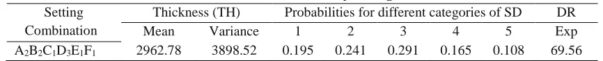
In the cells of Excel worksheet, the predicted values of mean, the variance of TH, and the expected value of DR at the chosen arbitrary setting combination are computed using regression Eqs. (16-18), respectively. On the other hand, the expected individual probabilities for each category of SD at the chosen setting combination are computed using Eqs. (19-24). The computed predicted values of mean and the variance of TH, the expected values of DR and the individual probability for each of the five categories of SD at the chosen arbitrary setting combination are given in Table 2.
Table 2. Predicted mean and variance of TH, probabilities for different categories of SD and the expected value of DR at the chosen arbitrary setting combination.
Setting Combination
Thickness (TH) Probabilities for different categories of SD DR
Mean Variance 1 2 3 4 5 Exp
A2B2C1D3E1F1 2962.78 3898.52 0.195 0.241 0.291 0.165 0.108 69.56
The predicted mean and the variance of TH are transformed into PRSNR
value (𝑃𝑅𝑆𝑁𝑅𝑇𝐻) using Eq. (9), and the expected values of DR is transformed into PRSNR value (𝑃𝑅𝑆𝑁𝑅𝐷𝑅) using Eq. (8). The computed 𝑃𝑅𝑆𝑁𝑅𝑇𝐻 and 𝑃𝑅𝑆𝑁𝑅𝐷𝑅 values are obtained as follows:
𝑃𝑅𝑆𝑁𝑅𝑇𝐻 = 10𝑙𝑜𝑔10
𝜇𝑇𝐻2
𝜎𝑇𝐻2
= 10𝑙𝑜𝑔10(
2962.782
3898.522) = 33.525
𝑃𝑅𝑆𝑁𝑅𝐷𝑅 = −10𝑙𝑜𝑔10
1
𝜇𝐷𝑅2 = −10𝑙𝑜𝑔10(
1
69.562) = 36.847
On the other hand, among different categories of SD, Category 1 is the most preferred one and Category 5 is the most undesirable one. Therefore, the weights 5, 4, 3, 2, and 1 are assigned to Categories 1, 2, 3, 4, and 5, respectively; the location score (W) and the dispersion score (d2) for SD are computed in Excel worksheet using Eqs. (13) and (14), respectively. The scores are obtained as 𝑊 = 3.251 and 𝑑2=18.019. Then, by putting the values of location and dispersion scores in Eqs. (15) and (16), the MSE and PRSNR values for SD at the chosen setting combination are obtained as follows:
𝑀𝑆𝐸𝑆𝐷≅ 1 𝑊2(1 +
3𝑑2
𝑊2) = 0.578
𝑃𝑅𝑆𝑁𝑅𝑆𝐷= −10𝑙𝑜𝑔10[ 1 𝑊2(1 +
3𝑑2
𝑊2)] = 2.378 ,
Finally, assuming equal weights for all the three quality characteristics TH, SD and DR, and the overall performance index (WPRSNR) is computed in Excel worksheet as follows:
𝑊𝑃𝑅𝑆𝑁𝑅 =1
WPRSNR is essentially a function of the control factor levels. So, the ‘Solver’ tool of Microsoft Excel optimization package is now applied to maximize this WPRSNR value by changing the level values of input variables (control factors). At optimizing, we have specified the integer restrictions for the level values of input variables mainly to make it comparable with the optimal solutions obtained by Wu [17]. The optimal setting combination of the control factors is obtained as A1B1C3D2E1F3.
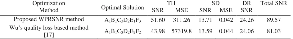
Wu [17] analyzed the same experimental data of Phadke [31], considering TH and DR as the quantitative response variables and SD as the ordinal response variable. He determined that A1B1C3D2E2F2 is the optimal factor level combination. For evaluating the optimization performance, the expected values of mean and the variance of TH, the expected probabilities for different categories of SD, and the expected values of DR under the two optimal process conditions are estimated; these values are presented in Table 3. Then, the total SNR values as well as the expected MSE values of individual response variables (except DR) under these two optimal conditions are computed. These computed values are shown in Table 4. As mentioned earlier, the lesser MSE values and the higher SNR values for the response variables are desirable. It may be observed from Table 4 that MSE values for TH and SD are smaller, and the total SNR value is higher under the optimal condition derived by the proposed WPRSNR method. This implies that the proposed WPRSNR method leads to better optimal solution.
Table 3.Expected values of different responses under the two optimal process conditions. Optimal condition
(Method)
TH Expected probabilities for different categories of SD
DR
Mean Variance 1 2 3 4 5 Exp.
value A1B1C3D2E1F3
(WPRSNR method) 3585.09 88.94 0.930 0.047 0.016 0.005 0.002 16.33
A1B1C3D2E2F2
(Wu’s method [17]) 3361.53 451.86 0.907 0.062 0.022 0.006 0.003 15.97
Table 4. Expected MSE and total SNR values under the optimal solutions obtained by the proposed WPRSNR method and Wu’s methods [17].
Optimization
Method Optimal Solution
TH SD DR Total SNR
SNR MSE SNR MSE SNR
Proposed WPRSNR method A1B1C3D2E1F3 51.60 311.26 13.71 0.042 24.26 89.57 Wu’s quality loss based method
[17] A1B1C3D2E2F2 43.98 57319.8 13.59 0.044 24.06 81.03
4.2 Case Study 2
categories of defect situation: Very good, good, and not good; not bad, bad, and very bad; those are denoted by grade I, II, III, IV, and V. Hsieh and Tong [29] considered six control factors A – F: Two levels for discrete control factor A and three levels for all other continuous control factors B-F. They carried out the experimentation using an L18 orthogonal array. There are two repetitions for IA. Depending on defect situation of 36 sensitive areas in a wafer, the DC response is categorized into five grades and the number of observations in each grade is listed. The experimental data obtained by Hsieh and Tong [29] have been presented in Table 5.
The same data are analyzed here using the proposed WPRSNR method. Since IA is a NTB type of quantitative response variable, its mean and variance are required to be estimated for computation of PRSNR value. Therefore, it is required to establish appropriate multiple regression equations for prediction of mean and variance of IA. In this experimental data, only two repetitive values are observed for IA. It is not appropriate to compute variance based on two values and fit the multiple regression equation based on those observed variance values. Therefore, it is decided to obtain regression equation only for the mean of IA. From the analysis of variance (ANOVA) table of this fitted mean model, an estimate of model error variance can be obtained. It is decided to use this model error variance for computation of PRSNR value. The fitted multiple regression equation for prediction of mean of IA is given in Eq. (25) along with
the R2andRadj2 values. The error variance of IA obtained by ANOVA table is found as 144.0.
Table 5. Experimental data on ion implantation process [29]. Expt
No.
Factors Ion amount (IA) Defect count (DC)
𝐸(𝑦𝐼𝐴) = −181.4 + 570.4𝐴 − 297.42𝐵 + 116.15𝐶 + 208.88𝐷 + 245.26𝐸 + 484.1𝐹 − 76.74𝐴𝐶
−149.48𝐴𝐷 − 35.86𝐴𝐸 + 72.2𝐵𝐶 − 106.06𝐶𝐹 − 104.6𝐸 [𝑅2= 0.996, 𝑅
𝑎𝑑𝑗2 = 0.994]
(25)
It is worth to mention that R2 and adjusted R2 values are very satisfactory for the multiple regression in Eq. (25). The results of various diagnostic checks for adequacy of the model are found satisfactory.
On the other hand, the ordinal response DC has 5 categories; therefore, the appropriate cumulative logit models are established for the first four categories of DC based on the computed cumulative probabilities in these categories. The established cumulative logit models for the first four categories are given in Eqs. (26-29).
𝑙𝑜𝑔𝑖𝑡[𝑃(𝐷𝐶 ≤ 𝐼)] = 3.4816 + 0.6359𝐴 − 1.478𝐵 − 1.14𝐶 + 0.265𝐷 − 0.1413𝐸 − 0.3194𝐹 (26)
𝑙𝑜𝑔𝑖𝑡[𝑃(𝐷𝐶 ≤ 𝐼𝐼)] = 4.6776 + 0.6359𝐴 − 1.478𝐵 − 1.14𝐶 + 0.265𝐷 − 0.1413𝐸 − 0.3194𝐹 (27)
𝑙𝑜𝑔𝑖𝑡[𝑃(𝐷𝐶 ≤ 𝐼𝐼𝐼)] = 5.818 + 0.6359𝐴 − 1.478𝐵 − 1.14𝐶 + 0.265𝐷 − 0.1413𝐸 − 0.3194𝐹 (28)
𝑙𝑜𝑔𝑖𝑡[𝑃(𝐷𝐶 ≤ 𝐼𝑉)] = 6.8474 + 0.6359𝐴 − 1.478𝐵 − 1.14𝐶 + 0.265𝐷 − 0.1413𝐸 − 0.3194𝐹 (29)
While the 𝑙𝑜𝑔𝑖𝑡 models for the first four categories are established, the cumulative probabilities up to the 𝑖𝑡ℎ(𝑖 = 𝐼, 𝐼𝐼, 𝐼𝐼𝐼, 𝐼𝑉)category can be computed using Eq. (30), and the individual probability for 𝑖𝑡ℎ(𝑖 = 𝐼, 𝐼𝐼, 𝐼𝐼𝐼, 𝐼𝑉, 𝑉) category can be obtained using Eq. (31).
𝑃(𝐷𝐶 ≤ 𝑖) = exp (𝑙𝑜𝑔𝑖𝑡[𝑃(𝐷𝐶 ≤ 𝑖)]
1 + exp (𝑙𝑜𝑔𝑖𝑡[𝑃(𝐷𝐶 ≤ 𝑖)] (30)
( 1), for 1
( ) ( ) ( 1), 2,3, 4
1 ( 4) for 5.
P DC i
P DC i P DC i P DC i i
P DC i
(31)
Now, the existing setting combination of input variable (control factors) A1B1C3D3E1F2 is chosen
as the starting combination of input variables for computational purpose. The expected value of IA at the chosen setting combination is computed using the regression of Eq. (25). On the other hand, the expected individual probabilities for each category of the ordinal variable DC at the chosen setting combination are also computed in cells of Excel worksheet using Eqs. (26-31). The expected value of IA and the individual probability for each category of DC at the chosen factor level combination are given in Table 6.
(27-30). The predicted value of IA and the individual probabilities of each category of DC at the chosen arbitrary setting combination have been given in Table 6.
Table 6. Predicted values of interest for IA and different categories of DC at the chosen process condition. Chosen Setting
Combination
Ion Amount (IA) Expected probabilities in different categories of DC Exp. value Variance I II III IV V A1B1C3D3E1F2 936.65 144.0 0.317 0.289 0.222 0.103 0.069
The predicted mean and the variance are transformed into PRSNR value (𝑃𝑅𝑆𝑁𝑅𝐼𝐴) using Eq. (9). The computed 𝑃𝑅𝑆𝑁𝑅𝐼𝐴 value is obtained as follows:
𝑃𝑅𝑆𝑁𝑅𝐼𝐴= 10𝑙𝑜𝑔10(
𝜇𝐼𝐴2
𝜎𝐼𝐴2) = 10𝑙𝑜𝑔10(
936.652
144 ) = 87.148
On the other hand, among different categories of DC, Category 1 is the most preferred one and Category 5 is the most undesirable one. Therefore, by assigning weights 5, 4, 3, 2, and 1 to Categories 1, 2, 3, 4 and 5, respectively, the location score (W) and the dispersion score (d2) for DC are computed using Eqs. (11) and (12), respectively. The obtained scores are 𝑊 = 3.6825 and 𝑑2=13.467. Then, by putting the values of location and dispersion scores in Eqs. (13) and (14), the MSE and PRSNR values for SD (𝑀𝑆𝐸𝐷𝐶and 𝑃𝑅𝑆𝑁𝑅𝐷𝐶) at the chosen setting combination are obtained as follows:
𝑀𝑆𝐸𝑆𝐷 ≅
1 𝑊2(1 +
3𝑑2
𝑊2) = 0.293
𝑃𝑅𝑆𝑁𝑅𝐷𝐶= 10𝑙𝑜𝑔10[
1 𝑊2(1 +
3𝑑2
𝑊2)] = 5.325
Finally, by assuming equal weights for the quantitative quality characteristics IA and the ordinal quality characteristics DC, the overall performance index (WPRSNR) is computed as follows:
𝑊𝑃𝑅𝑆𝑁𝑅 =1
2(𝑃𝑅𝑆𝑁𝑅𝐼𝐴+ 𝑃𝑅𝑆𝑁𝑅𝐷𝐶) = 46.24
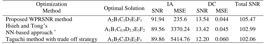
For the purpose of easy comparison of optimization performance, the expected values of IA and the probabilities in five categories of DC at the two optimal process conditions (A1B1C0.9D2.5E3F2 and A1B2C1D3E2F1) are reproduced from Hsieh and Tong [29] in Table 7.
Table 7. Expected values of measures at different optimal process conditions. Optimal conditions
(Method)
IA Exp. prob. in different categories of DC Exp. value 1 2 3 4 5 A2B1C1D3E3F1 (Proposed WPRSNR method)
1011.5 0.899 0.068 0.022 0.007 0.004 A1B1C0.9D2.5E3F2
(Hsieh and Tong’sapproach)* 1056.8 0.88 0.08 0.03 0.01 0.00 A1B2C1D3E2F1
(Taguchi method with trade off strategy) 1072.6 0.76 0.09 0.09 0.05 0.01
*Hsieh and Tong [29] did not impose integer restriction for the factor levels
For evaluating optimization performance, the total SNR values as well as the expected MSE values of individual response variables under these three optimal process conditions are computed. These computed values are presented in Table 8. As mentioned earlier, the lesser MSE values and the higher SNR values for the response variables are desirable. It is observed from Table 8 that the optimal process condition derived by the proposed WPRSNR method results in the highest total SNR value. Also, the expected MSE values of the individual response variables are the least under the optimal process condition derived by the proposed method. This implies that the proposed WPRSNR method leads to the best optimal solution.
Table 8. Expected MSE and total SNR values under the optimal solution obtained by the proposed WPRSNR method and Hsieh and Tong’s method [29].
Optimization
Method Optimal Solution
IA DC Total SNR
SNR MSE SNR MSE
Proposed WPRSNR method A2B1C1D3E3F1 91.94 235.6 13.54 0.044 105.47 Hsieh and Tong’s
NN-based approach * A1B1C0.9D2.5E3F2 89.56 3370.24 13.42 0.045 102.99 Taguchi method with trade off strategy A1B2C1D3E2F1 89.86 5414.76 12.20 0.060 102.06
*Hsieh and Tong [29] did not impose integer restriction for the factor levels
5. Discussions
to erroneous decision making about the out of control process condition. Therefore, further research is required for developing the appropriate methodology for simultaneous monitoring of quantitative and ordinal quality characteristics.
A limitation of the current research is that the demonstration of implementation of the developed method and evaluation of its usefulness have been carried out using the published experimental data in literature, i.e. secondary data. Thus, there is no scope for carrying out the confirmatory trials with the derived optimal factor-level combination. However, in both case studies, the optimal factor-level combinations derived by the proposed WRPSNR method results in the highest expected total SNR values and the lowest expected MSE values for the individual response variables. Therefore, it should not be inappropriate to consider that the results of analysis of the two case studies are indicative that the proposed WPRSNR method is very promising for simultaneous optimization of the quantitative and the ordinal response variables.
6. Conclusion
In real world, the overall quality of a product is often represented partly by the measured values of some quantitative variables and partly by the observed values of some ordinal variables. For ensuring the production of high quality products, the manufacturing process of a product needs to be optimized with respect to all these quantitative and ordinal response variables. In this article, a new approach for simultaneous optimization of the quantitative and ordinal responses was presented. In the proposed method, the relationship between an ordinal response variable and input controllable variables (control factors) was modeled by using the ordinal logistic regression and the relationship between a quantitative response variable; the input controllable variables were modeled by using the multiple regression. Then, a new performance metric, called the Weighted Predicted Response Based Signal-To-Noise Ratio (WPRSNR), was defined and optimized. Two well-known case studies in literature were analyzed using the proposed method. The comparison of results revealed that the proposed method led to the best optimal solution with respect to total SNR as well as MSE of the individual responses. A limitation of the current research is that it is carried out using secondary data and so, no confirmatory trials could be performed for validating the expected optimization performance. After optimization of the process settings, the process needs to be monitored continuously for ensuring the production of good quality product consistently. Therefore, the further research is required for developing the appropriate methodology for simultaneous monitoring of the quantitative and ordinal quality characteristics.
Acknowledgement
References
[1] Taguchi, G. (1986). Introduction to quality engineering. Tokyo, Asian Productivity Organization. [2] Derringer, G., & Suich, R. (1980). Simultaneous optimization of several response
variables. Journal of quality technology, 12(4), 214-219.
[3] Logothetis, N., & Haigh, A. (1988). Characterizing and optimizing multi‐response processes by the taguchi method. Quality and reliability engineering international, 4(2), 159-169.
[4] Vining, G. G., & Myers, R. H. (1990). Combining Taguchi and response surface philosophies: A dual response approach. Journal of quality technology, 22(1), 38-45.
[5] Tsui, K. L. (1999). Robust design optimization for multiple characteristic problems. International Journal of production research, 37(2), 433-445.
[6] Wu, F. C. (2004). Optimization of correlated multiple quality characteristics using desirability function. Quality engineering, 17(1), 119-126.
[7] Yin, X., He, Z., Niu, Z., & Li, Z. S. (2018). A hybrid intelligent optimization approach to improving quality for serial multistage and multi-response coal preparation production systems. Journal of manufacturing systems, 47, 199-216.
[8] Su, C. T., & Tong, L. I. (1997). Multi-response robust design by principal component
analysis. Total quality management, 8(6), 409-416.
[9] Tong, L. I., & Hsieh, K. L. (2000). A novel means of applying artificial neural networks to
optimize multi-response problem. Quality engineering, 13(1), 11–18.
[10] Tong, L. I., Wang, C. H., & Chen, H. C. (2005). Optimization of multiple responses using principal
component analysis and technique for order preference by similarity to ideal solution. The
International journal of advanced manufacturing technology, 27(3-4), 407-414.
[11] Liao, H. C. (2006). Multi-response optimization using weighted principal component. The
international journal of advanced manufacturing technology, 27(7-8), 720-725.
[12] Pal, S., & Gauri, S. K. (2010). Multi-response optimization using multiple regression–based
weighted signal-to-noise ratio (MRWSN). Quality engineering, 22(4), 336-350.
[13] Marcucci, M. (1985). Monitoring multinomial processes. Journal of quality technology, 17(2), 86-91.
[14] Franceschini, F., & Romano, D. (1999). Control chart for linguistic variables: A method based on the use of linguistic quantifiers. International journal of production research, 37(16), 3791-3801. [15] Wang, K., & Tsung, F. (2010). Recursive parameter estimation for categorical process
control. International journal of production research, 48(5), 1381-1394.
[16] Li, J., Tsung, F., & Zou, C. (2014). A simple categorical chart for detecting location shifts with ordinal information. International journal of production research, 52(2), 550-562.
[17] Wu, F. C. (2008). Simultaneous optimization of robust design with quantitative and ordinal data. International journal of industrial engineering: Theory, applications and practice, 15(2), 231-238.
[18] Karabulut, G. B. (2013). Comparison of methods for robust parameter design of products and processes with an ordered categorical response (Doctoral Dissertation, Middle East Technical University). Retrieved from http://etd.lib.metu.edu.tr/upload/12616313/index.pdf
[19] Box, G. (1986). Discussion of testing in industrial experiments with ordered categorical data by VN Nair. Technometrics, 28, 295-301.
[20] Hamada, M., & Wu, C. F. J. (1986). Discussion. Technometrics, 28(4), 302-306. [21] Agresti, A. (2010). Analysis of ordinal categorical data (Vol. 656). John Wiley & Sons.
[22] Nair, V. N. (1986). Testing in industrial experiments with ordered categorical data. Technometrics, 28(4), 283-291.
[24] Chipman, H., & Hamada, M. (1996). Bayesian analysis of ordered categorical data from industrial experiments. Technometrics, 38(1), 1-10.
[25] Jeng, Y. C., & Guo, S. M. (1996). Quality improvement for RC06 chip resistor. Quality and reliability engineering international, 12(6), 439-445.
[26] Wu, F. C., & Yeh, C. H. (2006). A comparative study on optimization methods for experiments with ordered categorical data. Computers & industrial engineering, 50(3), 220-232.
[27] Asiabar, M. H., & Ghomi, S. F. (2006). Analysis of ordered categorical data using expected loss minimization. Quality engineering, 18(2), 117-121.
[28] Bashiri, M., Kamranrad, R., & Karimi, H. (2012). Response optimization in ordinal logistic regression using heuristic and meta-heuristic algorithm. Journal of Sharif university, 28, 79-92.
[29] Hsieh, K. L., & Tong, L. I. (2001). Optimization of multiple quality responses involving qualitative and quantitative characteristics in IC manufacturing using neural networks. Computers in industry, 46(1), 1-12.
[30] León, R. V., Shoemaker, A. C., & Kacker, R. N. (1987). Performance measures independent of adjustment: an explanation and extension of Taguchi’s signal-to-noise ratios. Technometrics, 29(3), 253-265.
![Table 1. Summarized experimental data of polysilicon deposition process [31]. Exp no. Factors TH SD by categories DR](https://thumb-us.123doks.com/thumbv2/123dok_us/8580712.1718860/12.612.129.483.376.610/table-summarized-experimental-polysilicon-deposition-process-factors-categories.webp)
![Table 5. Experimental data on ion implantation process [29].](https://thumb-us.123doks.com/thumbv2/123dok_us/8580712.1718860/16.612.151.462.401.653/table-experimental-data-on-ion-implantation-process.webp)