An interactive approach for solving multi-objective nonlinear programming and its application to cooperative continuous static games

1. Introduction

objective analysis assumes that the objectives are generally in conflict. When modeling a Multi-Objective Linear Programming (MOLP) problem, how to calculate the exact values of the coefficients is a probabilistic task. Normally, the coefficients are either given by a Decision Maker (DM) subjectively or by statistical inference from historical data. Most multi-objective methods are based on interaction between a DM and the mathematical model of the problem under consideration. A typical interactive method exhibits a hierarchical structure composed of an analysis level, which comprises the solution of some auxiliary single objective optimization problem and decision level at which the DM tries to induce the analysis level to generate a solution that optimizes his (her) preference function [5]. Multi-objective optimization methods can be classified according to the DM influence in the optimization process [5]:

 Methods where DM does not provide information (no-preference methods).

 _{Corresponding author}

E-mail address: [email protected] DOI: 10.22105/jarie.2018.151038.1058

An Interactive Approach for Solving Multi-Objective Nonlinear

Programming and its Application to Cooperative Continuous

Static Games

Hamiden Abdelwahed Khalifa

Department Operations Research, Institute of Statistical Studies and Research, Cairo University, Giza, Egypt.

A B S T R A C T P A P E R I N F O

In this paper, an interactive approach for solving Multi-Objective Nonlinear Programming (MONLP) problem has introduced. This approach combines with the Reference Direction (RD) introduced by Narula et al. [10] and the Attainable Reference Point (ARP) method introduced by Wang et al. [17]. In the interactive approach, we still start with a weak efficient solution as the first step and use the corresponding objective values to improve the weighting coefficients of the augmented Lexicographic Weighted Tchebycheff Programming (LWTP) problem; hence we modify the reference point in the case of an unsatisfactory solution for the Decision Maker (DM) he (she) wishes. The cooperative continuous static game is introduced as an application and hence the stability set of the first kind is determined corresponding to its solution through the interactive approach. Finally, a numerical example has given to the utility of our interactive approach.

Chronicle:

Received: 03 September 2018 Revised: 14 November 2018

Accepted:13 August 2018

Keywords:

Multi-Objective Nonlinear Programming.

Efficient Solution. Reference Direction Method. Attainable Reference Point. Interactive Approach. Satisfactory Solution.

Cooperative Continuous Static Games.

Parametric Study.

Journal of Applied Research on Industrial

Engineering

 Methods where a posteriori information is used (posteriori methods).

 Methods where a priori information is used (priori methods).

 Methods where the progressive information is used (interactive methods).

Interactive approaches have been invented to combine advantages of both posteriori methods and priori methods and avoid the disadvantages. Since the DM is involved in the entire solution process, this approach has found better acceptance in practice. Among all the solution approaches, interactive methods have become popular and are considered promising for Multi-Objective Optimization Problems (MOPs). Although the numerous interactive procedures have been suggested, none has emerged as a clearly preferred approach [16]. Recently, researchers have introduced the concept of the algorithm which links various approaches in a way that make use of the advantages [4, 18]. A new algorithm for solving the MOP starting with the utopian point has been introduced by Sadrabadi and Sadjadi [15].

The applications of game theory may be found in economics, engineering, biology, and in many other fields. Three major classes of games are matrix games, continuous static games, and differential games. In continuous static games, the decision possibilities need not be discrete andthe decisions and costs are related in a continuous rather than a discrete manner. The game is static in the sense that no time history is involved in the relationship between costs and decisions. Elshafei [3] introduced an interactive approach for solving the Nash cooperative continuous static games and also determined the stability set of the first kind corresponding to the obtained compromise solution. Khalifa and ZeinEldein [6] introduced an interactive approach for solving cooperative continuous static games with fuzzy parameters in the objective function coefficients. Navidi et al. [11] presented a new game theoretic- based approach for multi response optimization problem. Osman et al. [14] introduced a new procedure for continuous time open loop stackelberg differential game. Khalifa [7] proposed an interactive approach for solving multi-objective nonlinear programming problem. The approach is based on the Reference Direction (RD) introduced by Narula et al. [10] and the Attainable Reference Point (ARP) method introduced by Wang et al. [17]. Cruz and Simaan [1] proposed the theory of ordinal games, where the players are able to rank-order their decision choices against the choice by the other players instead of payoff function objective functions. Muhammed et al. [9] conducted a review to investigate the various factors affecting cooperation in underwater acoustic sensor network. They studied the various cooperation techniques used for underwater acoustic sensor network from different perspectives. Molinac and Earn [8] investigated a type of public games played in groups of individuals who choose how much to contribute towards the product of a common good at the cost to themselves. The stability set gives a wide insight for the stability of the solution of parametric nonlinear optimization problems due to a parametric change. The essence of this approach is in the definition, characterization, and determination of a group of parameter sets, such as the set of feasible parameters, the solvability set, and the stability set of the first and second kinds. These sets have been defined and characterized in the crisp environment for parametric nonlinear differentiable programming problems by Osman [12] and Osman and Dauer [13].

2. Problem Formulation and Solution Concepts

Consider the following MONLP problem

1 2

minZ x( ) ( ( ), f x f ( ),...,x f_s( ) )x t

s.t. (1)

.

M

x



Where

x



R

n and

f

_i

(

x

),

i



1

,

2

,

3

,...,

s

are real valued functions. Is assumed that:

 The feasible region

M



R

n is non-empty and compact.



f

_i

(

x

),

i



1

,

2

,

3

,...,

s

, are continuous.

Definition 1. (Wang et al. [17]). Let f ( f₁,f₂,...,f_s)t be an attainable reference point, i.e.

s

i

f

f

_i



_i

,



1

,

2

,

3

,...,

and

f

may be feasible or infeasible for the Eq. (1), and

x

*



M

.

 *

x

is said to be reference non-dominated solution of MONLP problem if

x

*is an efficient solution of

MONLP Eq. (1), and

f

(

x

*

)



f

.

 A point

x

*is said to be reference (non-dominated) satisfactory solution of Eq. (1) if

x

* is reference

efficient solution and

f

(

x

*

)

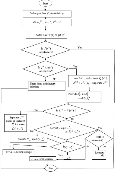
is satisfactory for the DM.

3. An Interactive Approach

The steps of the interactive approach

Step 1. Find



f as follows:

, max

,... 2 , 1

i m i

y



s.t. (2)

.

,

,

);

(

R

y

M

x

i

x

f

y

i i i









Step 2. Given an initial reference point

f

0



R

ssuch that

f

_i0



f

_i

. Let _I _{{1, 2,..., },s I}0 _I,h_0. Step 3. Calculate the weighting vector from the following relation

 

 

i h i i

f f

w 1

,

i



1

,

2

,

3

,

...,

s

,

₍₃₎















 





i i

s

i i s

i

f

x

f

Lex

min

,

(

)

1 ,...,

2 ,

1



s.t. (4)

.

0

,

,

...,

,

3

,

2

,

1

;

)

(

R

M

x

s

i

f

x

f

w

i i i i i















 





Let

x

hbe the obtained optimal solution.

Step 4: Determine the termination. When

f

h is satisfactory to the DM, stop with

x





x

h as the final solution. When

f

his not satisfactory and





h h

f

f

or hs, there is no satisfactory efficient reference solution of Eq. (1). Otherwise, go to Step 5.

Step 5: Modify the reference point. (i) DM selects any

e

_h in

J

hsuch that h

e

f

is an unsatisfactory objective in



f_i :iJh



at

f

h

.

Let

J

h1



J

h

/

{

e

_h

}.

Separate

J

h1 into two parts:



h i h i h h f f J i

J₁   1:  and DM wishes to release the value of

f

_i at

f

h



,

/

1

.

1 2 h h h

J

J

J



 (ii) For

h

J

i



₁ the DM provides



hi, the amount to be relaxed for

f

iat h

f

such that



ih



h i h

i



f



f



0

,

. Let

. 1 h i h i h i f

f    For

i



J

₂h

,

let 1 h.

i h

i f

f   For

i



J

h

/

J

h1, let 1 .

 

 _ h i h

i f

f (iii) In the case

h i h

i f

f 1  for all iJh/{e_h}, return to (i), to separate

J

h1 once again or return to (ii) to increase the amount to be relaxed for some ( 1)

h i i J

f  at

f

h, if the DM wishes to do so. Otherwise, stop and there is no satisfactory efficient solution. In the case that

f

_ih1



f

_ih for some

i



J

h

/

{

e

_h

}

, go to (iv)

Let , ' 1, h,

h i i

h f f i e

e

e    and solve the following auxiliary problem:

min

f

_e

(

x

)

s.t. (5)

e i s i f x

f_i( ) 'i, 1,2,..., , 

,

xM.

To get the solution

x

'h, when ( ' ) e ( h)

h

e x f x

f

h

h  or ( )

'h e x

f

h for objective

f

ehis not satisfactory to the DM, return to (ii) to increase the amount to be relaxed for some

f

_i

(

i



J

₁h

)

at

f

h, if the DM wishes to do so. Otherwise, stop there is no satisfactory efficient solution. When f_e (x'h) f_e (xh)

h

h  and

) ( 'h

e x

f

h for objective fehis satisfactory to the DM, he/ she provides ,

h e_h

 the largest amount to be improved for

h

e

f at

f

(

x

h

),

such that



0, ( ) e ( 'h)



h e h

e_h  f _h x  f _h x

 . Let 1 ( ) he .

h e h

e_h f _h x _h

f    (v) If

) ( '

1 h

e h

e f x

f

h

h 



i s i



,..., 2 , 1

min



s.t. (6)

.

0

,

,

...,

,

2

,

1

,

)

(

R

M

x

s

f

x

f

w

i i i i

i











 





Let hh1 and return to step (iii). If 1 e ( 'h),

h

e f x

f

h

h 



let hh1and return to Step 3.

Example 1. Consider the following problem:

T

x

f

x

f

x

Z

(

)

(

(

),

(

)

)

min



_{1 2}

s.t.

2 2

1 2 1 2

(x 3) (x 2) 0, 2x x 0.

Where

f

₁

(

x

)



x

₁ and

f

₂

(

x

)



x

₂.

Let us apply the steps of the interactive approach as:

Step 1. Starting with

x

 by solving the following problem:

i i 1,2



max



s.t.

1 1 2 2

2 2

1 2

1 2 ,

,

( 3) ( 2) 0,

2 0,

0 i , 1, 2.

x x

x x

x x

R i

 



 

   

 

  

Let the solution be

x





(

3

,

0019

,

1

.

9967

)

and the corresponding objective values are

).

9967

,

1

,

0019

,

3

(





f

Step 2. DM specifies an initial attainable reference point

f

_i



, such that 





_i

i

f

f

for every

i



1

,

2

that is

3

.

0004



f

1



5

.

0004

? 5.0004, and

1

.

9967



f

2



4

.

0004

? 4.0004. Then,

T

The following steps of the interactive approach has illustrated as in the following flowchart.

Step 3. Calculate the weighting vector from the following relation:

5004

.

0

1

1 1 1







_ 

f

f

w

, and 2

2 2 1 0.4991. w f f     

Step 4. Solve the problem through the LWTP Eq. (4) with the calculating weights as:

1 2

min {_i,x 3.0019x 1.9967 } s.t. . 0 , 0 , , 0 2 , 0 ) 2 ( ) 3 ( , 9967 . 1 4991 . 0 , 0019 . 3 5004 . 0 2 1 2 1 2 2 2 1 2 2 1 1 R x x x x x x x x i             







Step 5. Case1: x*(3.0019,0), f *(3.0019,0), f (5.0004,4,0004), and

)

9967

.

1

,

0019

.

3

(





f

is the DM satisfied Y/N: Y, stop with

x

*



(

3

.

0019

,

0

)

and

)

0

,

0091

.

3

(

*



f

as the final solution.

4. An Application in Cooperative Continuous Static Games

Consider the following Cooperative Continuous Static Game (CCSG), with parameters in the right hand side of the constraints, and with mplayers. These players respectively have the costs

   

 



,

,

,

,

...,

,



,

min

F

₁

a



F

₂

a



F

_m

a



(7)

s.t.

 

a j n

h_j ,



0, 1,2,..., (8)

 



Rk :g al( , ) l,l 1, 2,...,r



.

       (9)

Where

F

_i

,

i



1

,

2

,...,

m

are convex functions onR R gl l r

k n ..., , 2 , 1 , , 

 are concave functions on

k n

R

R



,



_lare any real numbers. Assume that there exists a function

a



f

(



).

If the functions

n

j

a

h

_j

(

,



),



1

,

2

,

...,

are differentiable then the Jacobin j k n a a h k j ..., , 2 , 1 , , 0 ) , (    



in a neighborhood of a solution point

(

a

,



)

to Eq. (8),

a



f

(



)

is the solution to Eq. (8) generated by

.











t m

F

F

F

(

),

(

),...,

(

)

min

₁'



₂'



'



s.t. (10)

r l

gl( ) l, 1,2,...,

'









.

Where F_i':Rk R,i1,2,...,mare convex functions on Rs,g_l' :Rk R,l1,2,...,r are concave functions on

R

,

F

i'

(



)

F

i'

(

f

(



),



),

k



and gl'(



)gl'(f(



),



). Here, we assume that Eq. (10) is

stable [2]. The proposed interactive procedure introduced in Section 3 is applied to the Eq. (10). Let



 be the final solution corresponding to







R

r obtain by solving Eq. (10) through the use of the proposed interactive procedure. To determine the stability set of the first kind corresponding to



 denoted by

S

(





)

, applying the following conditions:

l l l

l

u ( g ( ) ) 0, l 1,2,..., r

u 0, l 1,2,..., r.

_  _{ }

 

Example 2. Consider the following two player games with

F

₁'

(



)



(



₁



1

)

2



(



₂



1

)

2

,

F

₂'

(



)



(



₁



2

)

2



(



₂



2

)

2

.

Where player 1 controls



1



R

and player 2 controls



2



R

with

.

,

,

,

,

,

,

4

,

4

4 3 2 1

4 2

3 1

2 2

1 1

R











































By applying the proposed interactive approach to this problem we obtain the solution



0



(

0

.

6

,

1

.

85

)

corresponds to







(

2

,

2

,

0

,

0

)

T to determine

S

(

0

.

6

,

1

.

85

)

; we apply the following conditions:

. 0 ) 85 . 1 (

, 0 ) 6 . 0 (

, 0 ) 146 . 2 (

, 0 ) 4 . 3 (

4 4

3 3

2 2

1 1

  

  

 

  









u u u u

We have

I





1

,

2

,

3

,

4



.





1

4

1 2 3 4

(0.6, 1.85) : 3.4, 2.146, 0.6, 1.85

I

S  R          v   .

For I₂ 

 

2,4 , u₁0, u₂0, u₃0, u₄0.Then





2

4

1 2 3 4

(0.6, 1.85) : 3.4, 2.146, 0.6, 1.85.

I

S  R          v   .

For

I

₃





,

u

₁



0

,

l



1

,

2

,

3

,

4

.

Then





3

4

1 2 3 4

(0.6, 1.85) : 3.4, 2.146, 0.6, 1.85.

I

S  R          v   .

For I₄



1,2,3,4 ,



u₁0,l 1,2,3,4.Then





4

4

1 2 3 4

(0.6, 1.85) : 3.4, 2.146, 0.6, 1.85.

I

S  R          v   .

The stability set corresponding to the other proper subsets

I

qof



1

,

2

,

3

,

4



can be computed in the same

way. Hence,

S

(

0

.

6

,

1

.

85

)

is given by:

).

85

.

1

,

6

.

0

(

)

85

.

1

,

6

.

0

(

16

1 Iq

q

S

S







5. Conclusion

In this paper, an interactive approach for solving MONLP problems was proposed. This approach combined with the RD method introduced by Narula et al. [10] and the ARP method introduced by Wang et al. [17]. The advantages are the reduction of the number of iterations; hence the computational effort required to obtain the final solution was reduced. Also, the cooperative continuous static game was introduced as an application.

Acknowledgements

The authors are very grateful to the anonymous reviewers for his/her insightful and constructive comments and suggestions that have led to an improved version of this paper.

References

[1] Cruz, J. B., & Simaan, M. A. (2000). Ordinal games and generalized Nash and Stackelberg solutions. Journal of optimization theory and applications, 107(2), 205-222.

[2] Chankong, V., & Haimes, Y. Y. (2008). Multi-objective decision making: theory and methodology. Courier Dover Publications.

[3] Elshafei, M. M. K. (2007). An interactive approach for solving Nash cooperative continuous static games.

International journal of contemporary mathematical sciences, 2(24), 1147- 1162.

[4] Gardiner, L. R., & Steuer, R. E. (1994). Unified interactive multiple objective programming. European journal of operational research, 74(3), 391-406.

[6] Khalifa, H. A., & Zeineldin, R. A. (2015). An interactive approach for solving fuzzy cooperative continuous static games. International journal of computer applications, 113(1).

[7] Khalifa, H. A. (2016). An interactive approach for solving fuzzy multi-objective non-linear programming problems. The journal of fuzzy mathematics,3(24), 535- 545.

[8] Molina, C., & Earn, D. J. (2017). Evolutionary stability in continuous nonlinear public goods games. Journal of mathematical biology, 74(1-2), 499-529.

[9] Muhammed, D., Anisi, M., Zareei, M., Vargas-Rosales, C., & Khan, A. (2018). Game theory-based cooperation for underwater acoustic sensor networks: Taxonomy, review, research challenges and directions. Sensors, 18(2), 425.

[10]Narula, S. C., Kirilov, L., & Vassilev, V. (1994). An interactive algorithm for solving multiple objective nonlinear programming problems. In G. H. Tzeng H. F. Wang U. P. Wen & P. L. Yu (Eds.). Multiple criteria decision making (pp. 119-127). Springer, New York, NY.

[11]Navidi, H., Amiri, A., & Kamranrad, R. (2014). Multi-responses optimization through game theory approach. International journal of industrial engineering and production research, 25(3), 215- 224. [12]Osman, M. S. A. (1977). Qualitative analysis of basic notions in parametric convex programming. I.

Parameters in the constraints. Aplikace matematiky, 22(5), 318-332.

[13]Osman, M., & Dauer, J. (1983). Characterization of basic notions in multi-objective convex programming problems. Retrieved from Lincoln, University of Nebraska database.

[14]Osman, M. S., El-Kholy, N. A., & Soliman, E. I. (2015). A recent approach to continuous time open loop stackelberg dynamic game with min- max cooperative and non-cooperative followers. European scientific journal, 11(3), 94-109.

[15]Sadrabadi, M. R., & Sadjadi, S. J. (2009). A new interactive method to solve multiobjective linear programming problems. JSEA, 2(4), 237-247.

[16]Shin, W. S., & Ravindran, A. (1992). A comparative study of interactive tradeoff cutting plane methods for MOMP. European journal of operational research, 56(3), 380-393.

[17]Wang, X. M., Qin, Z. L., & Hu, Y. D. (2001). An interactive algorithm for multicriteria decision making: the attainable reference point method. IEEE transactions on systems, man, and cybernetics-part A: systems and humans, 31(3), 194-198.