A Comparative Study Of LRC, NNLS, Knn, And
Sparse Representation Based Classification Methods
Based On Audio Features
Nu War
University of Computer Studies (Banmaw), Mandalay, Myanmar, PH-+95 9 402656119
Abstract: Video comprises of two signal modes the acoustic and visual. The visual information is potentially more difficult to extract. In this work, only acoustic signal mode are considered and assessed for the task of genre classification. In the video genre classification field, there are many genres in the real world such as music, sport, information, education, news, and so on. In this paper, the three genres are only considered to classify such as cartoon, sport and music. The experiments with them have also provided a reference of the performance of such systems when dealing with the own video data set. Furthermore, it has been experimented with five classification methods (SRC, NNLS, LRC, MSRC, and kNN) in order to improve accuracy and to see relevant aspects and processes of them. It consists of discrete wavelet subband features, then computes the mean and variances for all. Furthermore, MFCC features are also implemented in feature extraction. Finally, a proper evaluation of the solution has been done. The overall accuracy and classification are also shown in the experimental results.
Keywords: MFCC, DWT, SRC, NNLS, LRC, MSRC, and kNN.
1.
Introduction
A typical, or even musically trained, person might have difficulty expressing a precise list of characteristics when asked to distinguish between two different sounds, even if he or she can easily differentiate between the sounds. Even when one is able to describe audio characteristics, these features are likely to be abstractions that are difficult to quantify and scientifically extract from audio signals. Unfortunately, high-level information such as this is currently difficult or impossible to reliably extract from general music signals. This difficulty means that one must at least start with low-level signal processing-oriented features. Determining which such low-level features are best-suited for any particular task can be difficult, as humans do not tend to think about sound in terms that are meaningful in a low-level signal processing sense. Fortunately, there are successful approaches to dealing with this problem. One can take an iterative approach to feature extraction, where low-level features derived directly from audio signals are used to derive mid-level representations, which can in turn be used to derive increasingly high-level features that are musically meaningful to humans. Although low-level features are not usually intuitive to humans directly, an individual well-trained in signal processing and in auditory perception can use his or her expertise to gain insights into when certain low-level features can be useful even on their own. Acoustic-space characterization is presented by using statistic classifier like gaussian mixture model (GMM), neural nets or support vector machines (SVM) on cepstral domain features [1, 2, 3]. Various kinds of acoustic features have been evaluated in the field of video genre identification. In [1, 3, 4], time-domain audio features are proposed like zero crossing rates or energy distributions. Therefore, low-level approaches present a better robustness to the highly variable and unexpected conditions that may be encountered on videos. In the cepstral domain, one of the main difficulties in genre identification is due to the diversity of the acoustic patterns that may be produced by each video genre. In this paper, this problem is aim to address in the field of
identifying video genres by applying either wavelet mean and variance features or MFCC features. Video genre classification framework is focused on by using an audio-only method. In the next section an overview of the presented system is provided first. The architecture of the system and the basic underlying concepts are explained. Secondly, the SRC classification algorithm is described. Finally, the experimental results are also shown with each genre classification results and analytical results.
2.
System Architecture
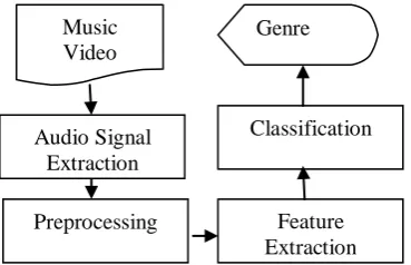
An automatic music video genre classification system is generally made up of three steps: preprocessing, feature extraction, and classification as shown in Figure 1. Music genre classifications that are studied and modelled include pop, rock and hip hop. The first process is the extracting audio information from a video clip. A stereo waveform should be converted into a mono waveform in the pre-process phase because this system is aimed to the mono waveforms.
Figure 1: The Overall Architecture of System
And then the features are extracted from an audio clip that is to be identified. The bark‟s scale wavelet is used to extract the audio feature. It is compact due to the wavelet property. It is informative due to the bark‟s scale property. The resulting wavelet features are used whenever it is desired to
Music Video
Preprocessing Feature
Extraction Classification
Genre
expand the database of known activities or to query the database when the clip is unknown. The final process is that of matching the new clips against the database to find a match, as well as testing the resulting match to ensure accuracy. A way of comparing features that is a similarity measure is therefore needed. Since the number of features comparisons is high in a large database and the similarity can be expensive to compute, methods that speed up the search are required. The identification results of each classification can be compared with time and accuracy.
2.1 Preprocessing
The input audio signal is digitized and converted to a certain format. It is resampled at 22 kHz for the mel scale with (16 bits per sample). This also involves averaging channels so that the signal is in mono when the signal is in stereo. A stereo waveform should be converted into a mono waveform in the pre-process phase because this proposed algorithm is aimed to the mono waveforms. This step is needed for the following steps to work properly because some audio signal might suffer from changes such as amplitude change, resolution change, resampling, filtering, noise addition, etc. Moreover, it can improve the efficiency of the algorithm and obtain a better model of the audio signal. To treat the signal as stationary to perform analysis on it, the signal is split up into short duration frames. The frames give a small window at which to look at the signal, over which the signal is treated as stationary. Therefore, the signal is divided into frames of a size comparable to the variation velocity of the underlying acoustic events. Overlap helps deal with window artifacts and non stationary channel noise. There is a trade-off between the robustness to shifting and the computational complexity of the system: the higher the frame rate, the more robust to shifting the system is but at a cost of a higher computational load. The length of an overlapping frame is 0.37 seconds with an overlapping factor of 27/32. The basic unit for identification is a block corresponding to 1 seconds of audio.
2.2 Wavelet Feature extraction
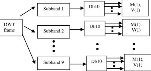
The human ear perceives better the lower frequencies than the higher ones. The spectral masking properties of human ear and the most natural subband decomposition is Bark frequency scale. The wavelet tree structure of Bark-scale wavelet decomposition is used to mimic the time-frequency analysis of the critical subbands according to the hearing characteristics of human cochlea. Critical subband is widely used in perceptual auditory modeling. The main drawback of the octave-band tree structure is that does not provide a good approximation of the critical subband decomposition of the human auditory system. The wavelet representation uses a wavelet transform to create a range of wavelets that allows examination of frequency components on a suitable scale. Therefore the input audio signal is decomposed into 19 critical wavelet subband signals by using Bark-scale wavelet decomposition that is implemented with an efficient nine-level tree structure. The decomposition process can be iterated, with successive approximations being decomposed in turn, so that one signal is broken down into many lower-resolution components. The wavelet feature of input audio signal is obtained by using the high-pass filter and low-pass filter, implemented with the Daubechies family wavelet (Db10). The DWT analysis can be performed using a fast, pyramidal algorithm related to multirate filterbanks [5]. To
obtain a useful feature extraction in this system, a mean and variance method is applied. For the nth frame, the mean and variance of βth subband is calculated by using subband detail coefficients as shown in Figure 2.
Figure 2: Feature Extraction by using Mean and Variance method
In the following expressions, β is the subband signal and (βi) the coefficient of β is an orthonormal basis. The mean and variance equation is as follow
M
Mean
M
m m
1)
(
(1)So, the variance of β-th
subband is calculated as
( ) ∑ ( ( ))
(2)
Features are extracted from each frequency band of every frame.
2.3 MFCC Feature Extraction
Other frequency related features are based on a preliminary Fast Fourier Transformation (FFT) to obtain a representation of the audio signal in the frequency domain. Such approaches assume that the signal is periodical. To avoid border effects each window is typically weighted with a Hann filter in order to attain that the values of both borders are zero. The frequency spectrum calculated with the magnitudes of the frequencies that are sampled by the FFT. This can be interpreted as an empirical probability distribution in the frequency space from which other data features are derived. The frequency spectrum as obtained by the FFT has a rather high resolution of frequency bins and puts equal emphasis on all frequency ranges. Motivated by the success in speech recognition music researchers have used psycho-acoustic transformations of the spectral content to summarize frequencies into larger bins (so-called bands) and emphasize frequency ranges that the human ear is most sensitive to. Human Auditory system behavior can be modeled by a set of critical band filter. The Mel bands are one of these. It is based on the Mel frequency scale, which is linear at low frequencies (below 1000 Hz). The Mel scale is especially popular in the Automatic Speech Recognition community where it is used for the calculation of the Mel Frequency Cepstral Coefficient (MFCC). The MFCC represent the shape of the spectrum with very few coefficients. First a discrete Fourier transform (DFT) is applied to a short time frame of the time domain signal and the magnitude terms obtained. The second step is to apply a log function to the magnitude spectrum. This serves to
DWT frame
Subband 1
Subband 2
Subband 9
Db10 M(1),
V(1)
Db10 M(1),
V(1)
Db10 M(1),
reduce the dyamic range of the spectrum. Then a mel filter bank is applied and finally a discrete cosine transform (DCT) is applied to give the cepstral coefficients. The cepstrum, is the Fourier Transform (or DCT) of the logarithm of the spectrum. The Mel-cepstrum is the cepstrum computed on the Mel-bands instead of the Fourier spectrum. The use of mel scale allows better to take into account the mid frequencies part of the signal. The MFCC are the coefficients of the Mel cepstrum. The first coefficient being proportional to the energy is not stored; the next coefficients are stored for each frame. The so-called Mel Frequency Cepstral Coefficients (MFCC) are obtained from the Mel spectrum by applying the Discrete Cosine Transform (DCT).
Nn n k
k
k
N
N
k
n
x
w
y
1
,...,
1
,
2
)
1
)(
1
2
(
(3)
N
w
1
1
(4)
N
k
N
w
k,
2
,...,
2
(5) where k is the index of the DCT coefficient and
)'
,...,
(
x
1x
Nx
is the N-vector of the logarithms of the amplitudes measured by the Mel band filters. The resulting series of coefficients is called the cepstrum (an anagram of spectrum). Sometimes the Inverse Fourier Transform is used instead of the DCT. The time series of the first 20 MFCC are calculated from each spectrum. This transformation decorrelates the time series similar to applying principal component analysis but has the advantage to be independent of the data. The resulting series of coefficients is called the cepstrum (an anagram of spectrum). Sometimes the Inverse Fourier Transform is used instead of the DCT. The time series of the first 20 MFCC are calculated from each spectrum. This transformation decorrelates the time series similar to applying principal component analysis but has the advantage to be independent of the data. In the next section, the classification method of the proposed recognition system is explained to recognize music video genre.3.
Classification
For the classification, the supervised sparse representation SR based classification algorithm is applied, as sufficient data is available for training and testing. It is believed that the sparsely constraint will make the coding vector more discriminative so that the classification accuracy can be improved. Sparse representation by -norm minimization is robust to noise, outliers and even incomplete measurements and SR has been successfully used for classification. It is widely used for different applications, such as signal separation, denoising, image inpainting, robust classification, inducing similarity measurement and shadow removal. In this paper, it is compared with the five types of classification methods: Sparse representation based classification (SRC) [6, 7], Non-negative Least Square classification (NNLS) [8], Linear regression based classification(LRC) [9], Meta-sample based SR classification (MSRC)[10], and kNN.
3.1 kNN
kNN has been applied to video genre classification since the early stages of the research. The k-nearest neighbors (k-NN) algorithm is a simple non-parametric classification algorithm. Despite its simplicity, it can give competitive performance compared to many other methods. It is widely used in machine learning and has numerous variations[12,13,14]. Given a test sample of unknown label, it finds the k-NN in the training set and assigns a label to the test sample according to the labels of those neighbors. The kNN algorithm is quite simple: given a test input data, the system finds the k nearest neighbors among the training features, and uses the categories of the k neighbors to weight the category candidates. The similarity score of each neighbor feature to the test feature is used as the weight of the categories of the neighbor feature. If several of the k nearest neighbors shares a category, then the per-neighbor weights of that category are added together, and the resulting weighted sum is used as the likelihood score of that category with respect to the test features. By sorting the scores of candidate categories, a ranked list is obtained for the test data.
3.2 Linear Regression
In linear regression, the relationships are modeled using linear predictor functions whose unknown model parameters are estimated from the data. Most commonly, the conditional mean of the response given the values of the explanatory variables (or predictors) is assumed to be an affine function of those values; less commonly, the conditional median or some other quantile is used. Like all forms of regression analysis, linear regression focuses on the conditional probability distribution of the response given the values of the predictors, rather than on the joint probability distribution of all of these variables, which is the domain of multivariate analysis. In statistics, linear regression is a linear approach to modeling the relationship between a scalar response (or dependent variable) and one or more explanatory variables (or independent variables). The case of one explanatory variable is called simple linear regression. For more than one explanatory variable, the process is called multiple linear regression. This term is distinct from multivariate linear regression, where multiple correlated dependent variables are predicted, rather than a single scalar variable.
3.3 Non-Negative Least Square
In mathematical optimization, the problem of non-negative least squares (NNLS) is a type of constrained least squares problem where the coefficients are not allowed to become negative. That is, given a matrix A and a (column) vector of response variables y, the goal is to find
‖ ‖ (5)
Here means that each component of the vector x should be non-negative, and ‖ ‖ denotes the Euclidean norm. From [11], the SRC, MSRC, LSRC classification methods confirms the good performance of human identification system except NNLS but it is still reasonable results.
3.4 Sparse Representation
data is available for training and testing. There are two key points in SRC [15]. The first key point is that encodes a query sample as a linear combination of a few atoms from a predefined dictionary, and the second key point is that the coding of y is performed collaboratively over the whole dataset X instead of each subset Xi. The SRC does not contain separate training and testing stages to be the over-fitting problem is much lessened. The SRC algorithm can be summarized as below:
Input: matrix of training samples for k classes; testing sample
Step 1. Normalize each column of A to unit -norm; Each column of A is required to be unit -norm in order to avoid trivial solutions that are due to the ambiguity of the linear reconstruction.
Step 2. Solve the − norm minimization problem ̂
‖ ‖ The second step which is used to calculate the sparse representation where is − norm which is equivalent to the number of non-zero components in the vector x.
Step 3. Compute the residual ( ) ‖ ( ) ( ̂)‖ , for i = 1, ..., c, where is the characteristic function that selects the coefficients associated with the ith class;
Step 4. Identify ( ) ( ) , where I(y) stands for finding the class label of y.
In this method, a testing sample is represented as the linear combination of the original training samples, and the representation error over each class is used as an indicator to classify the testing sample. The success of this technique is partially due to its robustness to noise and missing data.
3.5 Meta-Sampled Sparse Representation
As the common point of SRC and MSRC, the coefficient vector is used for classification or clustering. As the different point, MSRC is represented as a linear combination of metasamples which is extracted in a supervised manner from each class separately. In meta-sample based clustering, each sample is represented as a linear combination of meta-samples. A set of meta-samples are extracted from the training samples, and then an input testing sample is represented as the linear combination of these meta-samples by -regularized least square method. Classification is achieved by using the coefficient vector for the meta-samples extracted from each category, which is obtained by l1-regularized least square. In MSRC, it is expected that a testing sample can be well represented by using only the training samples from the same class. It does not contain the separate training and testing stages so that the over-fitting problem is much lessened more detail in [7].
4.
Experiment
For all the experiments described in this paper, a unique environment is created. Processing times are measured on Intel® Core™i3-3120M CPU running at a clock rate of 2.50 GHz with 4.00 GB of RAM on a Windows platform laptop. All of the music genre classification system is developed using Matlab environment. In setting up the experiment data, the average video length in the collection is 240 seconds (4 minutes). These video clips were taken from youtube, internet or CD albums such as cartoon, sport and music. With such a collection it would also be possible to create
correct identification results of the system. Tests were performed using a 4 fold cross-validation approach. Experiments were repeated for different combinations between training and testing. In this paper, the system is tested by randomly splitting the data set into training and test sets. Using the dataset that includes the wavelet mean & variance features and MFCC features, the classification scheme is implemented the five classifiers that discussed in the above section.
4.1 Analysis of Wavelet Features
In the analysis of feature sets, datasets and classifiers, it will be shown the average accuracy percentage of ten times testing on each classifier and each dataset.
Table 1: Classification Accuracy of Wavelet Means Features
Size of Dataset
150 dataset
(%)
601 dataset (%)
745 dataset
(%)
985 dataset
(%) Classifiers
kNN 34.57 34.59 39.70 36.94
SRC 33.54 35.72 38.68 38.89
NNLS 40.26 41.39 41.84 41.28
LRC 30.92 32.47 33.53 34.50
MSRC 31.12 36.73 33.48 37.87
Table 1 shows the accuracy result of wavelet mean features with the different size of dataset. From this table, wavelet mean feature has not sufficient qualities in this video music classification system. All classifiers give the accuracy result below the 50%. Among them, NNLS give the highest accuracy rate.
Table 2: Classification Accuracy of Variance Features
Size of
Dataset dataset 150 (%)
601 dataset (%)
745 dataset
(%)
985 dataset
(%) Classifiers
kNN 69.89 70.33 68.17 66.44
SRC 72.81 79.04 70.75 67.37
NNLS 67.53 68.13 71.61 60.22
LRC 51.22 37.86 42.03 41.24
MSRC 73.54 60.89 59.31 49.66
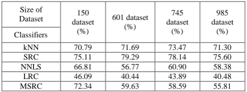
Table 3: Classification Accuracy of Combination of Means & Variance Features
Size of
Dataset dataset 150 (%)
601 dataset (%)
745 dataset
(%)
985 dataset
(%) Classifiers
kNN 70.79 71.69 73.47 71.30
SRC 75.11 79.29 78.14 75.60
NNLS 66.81 56.77 60.90 58.38
LRC 46.09 40.44 43.89 40.48
MSRC 72.34 59.63 58.59 55.81
form dataset to 745-dataset, SRC is increased from 150-dataset to 601 150-dataset. In the testing with 745-150-dataset, almost all classifiers give the best accuracy in music video classification system. In biggest dataset of this paper, the accuracy of all classification method is slightly fall back. LRC is poor classification method in this experiment.
Table 4: Classification Time of Combination of Means & Variance Features
Size of
Dataset dataset 150 (s)
601 dataset (s)
745 dataset
(s)
985 dataset (s) Classifiers
kNN 0.003 0.172 0.131 0.1348
SRC 4.39 34.95 50.02 80.08
NNLS 0.268 32.73 88.03 321.99
LRC 0.039 0.275 0.354 0.5549
MSRC 2.040 7.82 10.08 14.39
According to the Table 4, the lowest classification time of classifiers is kNN. Although the size of dataset is bigger and bigger, it can maintain the stability of classification time within 1s. So do LRC. In SRC, the classification is steadily increasing with the size of dataset. The classification time is about 1.33 minutes in the experiment with the biggest dataset of this paper. In the worst case, the NNLS takes the time over 5 minutes for the dataset(985 clips).
Table 5: Classification Time of Variance Features (s)
Size of
Dataset 150 dataset (s)
601 dataset (s)
745 dataset
(s)
985 dataset
(s) Classifiers
kNN 0.003 0.113 0.115 0.119
SRC 4.202 28.34 35.40 64.65
NNLS 0.319 41.75 107.86 369.94
LRC 0.024 0.123 0.1563 0.2414
MSRC 1.796 7.310 9.517 12.028
From Table 4 and Table 5, the size of feature set become large and tend to increase the classification time. The fraction of time devoted to combining feature is (eg. 80.08/64.6543) is 1.24 percent –a negligible amount. Thus the feature combination method is used in this music video classification system for the better accuracy.
4.2 Analysis of MFCC Features
In this section, datasets and classifiers, it will be shown the average accuracy percentage of ten times testing on each classifier and each dataset.
Table 6: Classification Accuracy of MFCC Features
Size of
Dataset 150 dataset (%)
601 dataset (%)
745 dataset
(%)
985 dataset
(%) Classifiers
kNN 93.95 81.78 81.49 81.76
SRC 95.26 84.77 83.37 84.53
NNLS 94.74 60.24 66.26 61.21
LRC 29.47 29.19 38.89 41.51
MSRC 80.00 58.39 64.92 66.16
After examine Table 1, Table 2, Table3 and Table 6, the wavelet mean feature is much simple but also much lower
accuracy than the variance of wavelet features. Moreover, the gap between the accuracy of wavelet variance feature and that of MFCC features is very high. Thus the most meaningful feature for audio based video genre classification system is MFCC features.
Table 7: Classification Time of MFCC Features
Size of
Dataset 150 dataset (s)
601 dataset
(s)
745 dataset
(s)
985 dataset
(s) Classifiers
kNN 0.1270 0.1594 0.1294 0.1327
SRC 3.5367 28.592 38.4746 54.8317
NNLS 0.3664 32.0039 77.7068 249.7844
LRC 0.0545 0.2756 0.3636 0.5335
MSRC 1.9660 8.2336 9.1996 11.9857
According to Table 7, if the size of dataset is too large, excessive classification time results in all classification methods except kNN classifier. In all classifiers except LRC from Table 6 and Table 7, if the size of dataset is too small, the classification accuracy become very large and tend to reduce the classification time.
4.3 Identification of Genre Using MFCC Feature
In this section, there is shown the classification result of each genre with the table of confusion matrix. All of confusion matrix is test with the 745 datasets. Because of four fold cross validation method, the training set is 558 and the testing set is 187.
Table 8: Confusion Matrix for kNN classifier
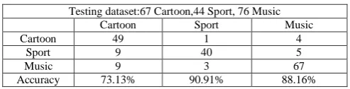
Table 9: Confusion Matrix for SRC classifier
Testing dataset:67 Cartoon,44 Sport, 76 Music
Cartoon Sport Music
Cartoon 54 1 4
Sport 2 41 2
Music 11 2 70
Accuracy 80.60% 93.18% 92.11%
Table 10: Confusion Matrix for NNLS classifier
Testing dataset:67 Cartoon,44 Sport, 76 Music
Cartoon Sport Music
Cartoon 40 4 11
Sport 15 31 7
Music 12 9 58
Accuracy 59.70% 70.45% 76.32%
Table 11: Confusion Matrix for MSRC classifier
Testing dataset:67 Cartoon,44 Sport, 76 Music
Cartoon Sport Music
Cartoon 36 2 11
Sport 15 39 19
Music 16 3 46
Accuracy 53.73% 88.64% 60.53%
Testing dataset:67 Cartoon,44 Sport, 76 Music
Cartoon Sport Music
Cartoon 49 1 4
Sport 9 40 5
Music 9 3 67
Table 12: Confusion Matrix for LRC classifier
Testing dataset:67 Cartoon,44 Sport, 76 Music
Cartoon Sport Music
Cartoon 35 33 21
Sport 15 9 18
Music 17 2 37
Accuracy 52.23% 20.45% 48.68%
From Table 8 to Table 12, this results are the best one time of ten times 4-cross validation. The overall accuracy of kNN, SRC, NNLS, LRC, MSRC is 83.42%, 88.24%, 68.98%, 43.32%, and 64.71%, respectively. All of these results are tested with only MFCC features. In kNN and SRC give the good hit rate for all three genre types. In sport type, all classifiers give the highest accuracy rate among all genre types except LRC.
5.
Conclusion
Video genre identification is still a reduced area of research, but the results obtained in it can be of great importance for closely related fields such as video segmentation, telemedicine cognition and perception, and many others. A good classification method should achieve a balance between two extremes that are the classification time and accuracy. Although the SRC is the best classification method in the point of view of accuracy, it is rising the classification time with the increasing size of dataset. The kNN is the good classification method in the both of time and accuracy. Only variance of wavelet features clearly demonstrates that a saving in disk and memory space can be achieved. The wavelet mean and variance features set offers the good classification accuracy in kNN and SRC method but their correct rates are only 73.47% and 79.39% respectively. Thus it can be concluded that the wavelet mean and variance features is not robust in music video classification system. The goal of paper is to provide adequate method with an acceptable level of performance. It can be achieved this goal by employing MFCC features in the audio based-video genre classification.
References
[1] M. Roach, L.-Q. Xu, and J. Mason, “Classification of non-edited broadcast video using holistic low-level features,” (IWDC„2002), 2002.
[2] R. Jasinschi and J. Louie, “Automatic tv program genre classification based on audio patterns,” in Euromicro Conference, 2001, 2001.
[3] L.-Q. Xu and Y. Li, “Video classification using spatial-temporal features and pca,” in Multimedia and Expo, (ICME „03), 2003.
[4] M. Roach and J. Mason, “Classification of video genre using audio,” in European Conference on Speech Communication and Technology, 2001.
[5] S. G. Mallat and W.L. Hwang, “Singularity Detection and Processing with wavelets,” IEEE Transactions on Information Theory, 38 (2): 617-643, 1992.
[6] C-P.Wei, Y-W.Chao, Y-R.Yeh,and Y-C. F.Wang, “Locality-sensitive dictionary learning for sparse
representation based classification”, Pattern Recognition 46 (2013) 1277–1287.
http://dx.doi.org/10.1016/j.patcog.2012.11.014
[7] L. Zhanga, M.Yanga, and X.Fengb, “Sparse Representation or Collaborative Representation: Which Helps Face Recognition? ”
[8] Boutsidis, Christos; Drineas, Petros (2009). "Random projections for the nonnegative least-squares problem". Linear Algebra and its Applications. 431 (5–7): 760– 771. doi:10.1016/j.laa.2009.03.026.
[9] C-G.Li, J.Guo and H-G.Zhang, “Local Sparse Representation based Classification”, 2010 International Conference on Pattern Recognition.
[10]C-H. Zheng , L.Zhang, T-Y.Ng, and C.K.Shiu, “Metasample Based Sparse Representation for Tumor Classification”.
[11]N. N. Htwe, and N. War, “ Human Identification Using Biometric Gait Features,” International Conference on Advances in Engineering and Technology (ICAET'2014) March 29-30, 2014.
[12]K. Z. Thwe, N. War, “Environmental Sound Classification using Time-frequency Representation”, IEEE/ACIS International Conference on Software Engineering, Artificial Intelligence, Networking and Parallel/Distributed Computing (SNPD 2017) ; Date- June 26-28, 2017, Kanazawa, Japan. ISBN: -0585-1-879
0055 -3
[13]K. Z. Thwe, N. War, “Local Tetra Pattern Texture Features for Environmental Sound Event Classification”, The 18th International Conference on Parallel and Distributed Computing, Applications and Technologies (PDCAT'17), 2017, Taipei Taiwan. [14]T. T. Yu, N. War, “Condensed Object Representation
with Corner HOG Features for object Classification in Outdoor Scenes”, IEEE/ACIS International Conference on Software Engineering, Artificial Intelligence, Networking and Parallel/Distributed Computing SNPD 2017, Kanazawa, Japan.
[15]T. Guha and R. K. Ward, Fellow, “Learning Sparse Representations for Human Action Recognition”, IEEE Transactions on Pattaern analysis and Machine Intelligence, VOL. , NO. , July 2011.