Canonical duality theory and triality for solving general global optimization problems in complex systems

COPYRIGHT NOTICE

FedUni ResearchOnline

http://researchonline.federation.edu.au

This is the published version of the following article:

Morales-Silva, D., Gao, D. (2015) Canonical duality theory and triality for solving

general global optimization problems in complex systems. Mathematics and

Mechanics of Complex Systems, 3(2), pp. 139-161.

Copyright © 2015, Mathematical Sciences Publishers.

This is the published version of the work. It is posted here with the permission of the publisher for your personal use. No further use or distribution is

Vol. 3, No. 2, 2015

dx.doi.org/10.2140/memocs.2015.3.139

M M∩

CANONICAL DUALITY THEORY AND TRIALITY

FOR SOLVING GENERAL GLOBAL OPTIMIZATION PROBLEMS IN COMPLEX SYSTEMS

DANIEL MORALES-SILVA AND DAVIDY. GAO

General nonconvex optimization problems are studied by using the canonical duality-triality theory. The triality theory is proved for sums of exponentials and quartic polynomials, which solved an open problem left in 2003. This theory can be used to find the global minimum and local extrema, which bridges a gap between global optimization and nonconvex mechanics. Detailed applications are illustrated by several examples.

1. Introduction and motivation

This paper intends to solve the following nonconvex optimization problem ((P)in short): (P):ext 5(x)=W(x)+1 2x t_{Ax− f}t_x:x∈ Rn , (1) where ext{ · }_{denotes finding extremum points of a function given in}{ · }_{, f} ∈_Rn is a given (input) vector, A∈_Rn×n_{is a given symmetric matrix, and}W:_Rn→_Ris a combination of fourth-order polynomials (double-well functions) and quadratic-exponential functions, namely

W(x):=X i∈Im exp 1₂xtBix−α_i+X j∈Ip 1 2bj 1 2x t_Cjx−θ j 2 ,

where Im= {1, . . . ,m}and Ip= {1, . . . ,p}are two integer sets withmand pthat are fixed integers; all the coefficients bj with j∈ Ip are positive constants, and

αi, θj ∈R for alli ∈ Im and j ∈ Ip are given parameters; the matrices{Bi}i∈Im

and{_Cj}_j∈Ip are assumed to be symmetric, positive semidefinite such that the cone

generated by them contains a positive-definite matrix.

The nonconvex optimization problem(P)arises naturally in complex systems with a wide range of applications, including chaotic dynamical systems[Gao 2003a;

Gao and Ogden 2008a;Gao and Ruan 2008], computational biology[Zhang et al. Communicated by Martin Ostoja-Starzewski.

MSC2010: 49N15, 90C26.

Keywords: canonical duality, triality theory, nonlinear analysis, nonconvex optimization, complex systems.

2011], chemical-database analysis[Xie and Schlick 2000], large-deformation com-putational mechanics[Gao 1996;Santos and Gao 2012], population growing[Ruan and Gao 2014a], location/allocation, network communication[Gao et al. 2012], and transitions of solids [Gao and Ogden 2008a;2008b;Gao and Yu 2008], etc.

For example, the popular sensor-network location problem is to solve the follow-ing system of nonlinear equations (see[Aspnes et al. 2004;Moré and Wu 1997]):

kui−ujk2₂=di j2 ∀(i, j)∈Ip, uk =ak ∀k∈Ib, (2) where the vectors ui = {uα_i} ∈ _Rd _(i =₁, . . . ,_{p) represent the locations of the} unknown sensors,Ip= {(i, j):i< j, di j is specified}and Ib= {k :uk=ak is specified}_{are two given index sets,}di j are given distances for(i, j)∈Ip, and the given vectorsa1,a2, . . . ,aq∈Rdare the so-called anchors. The notationkui−ujk2 denotes the Euclidean distance betweenui anduj; i.e.,

kui−ujk2= s d P α=1 (uα_i −uα_j)2.

By using the least-squares method, the quadratic equations(2)of the sensor-localiz-ation problem can be reformulated as an optimizsensor-localiz-ation problem:

min P(u)= X (i,j)∈I_p 1 2 kui−ujk 2 2−di j2 2 :_ui ∈U_a , (3)

whereUa= {u∈Rd×p:uk=ak∀k∈Ib}is a feasible space. Letx= {{u1₁, . . . ,ud₁},

. . . ,{u1_p, . . . ,ud_p}} ∈_Rn (n = d× p) denote an extended vector. By using the Lagrange-multiplier method to relax the boundary conditions in Ua, the least-squares method for the sensor-localization problem(3)can be written in the prob-lem(1)for certain properly defined matrices{_Cj}_{, which are the so-called} deforma-tion matrices in structural mechanics. The sensor-network-localizadeforma-tion-type prob-lems also appear in computational biology, Euclidean ball packing, molecular con-firmation, recently wireless network communication, etc.[Ruan and Gao 2014b;

Zhang et al. 2011]. Due to the nonconvexity, the sensor-network localization prob-lem is considered to be NP-hard even for the simplest cased=_{1[Moré and Wu}

1997;Saxe 1979]. A recent result of Aspnes et al.[2004]shows that the problem of computing a realization of the sensors on the plane is NP-complete in general.

Mathematics and mechanics have been complementary partners since Newton. Many fundamental ideas, concepts, and mathematical methods extensively used in calculus of variations and optimization originated from mechanics. For example, the Lagrange-multiplier method was first proposed by Lagrange from the classical analytic mechanics while the concepts of superpotential and subdifferential in mod-ern convex analysis were introduced in[Moreau 1968;Moreau et al. 1988]from

frictional mechanics. From the point of view of computational large-deformation mechanics, both the fourth-order polynomial-minimization problem(P)and the sensor-localization problem(3)are actually two special cases of discretized finite-deformation problems[Gao 1996]. It is known that, in continuum mechanics and differential geometry, the deformationu(x):→_Rr is a vector field over an open domain⊂_Rr_{, and the minimal-potential variational problem is defined by}

min P(u)= Z  [W(∇_u)−_uT _f]_d:_u∈U_a , (4)

whereW(F)is the so-calledstored strain energy, which is usually a nonconvex function of the deformation gradient F= ∇u, the feasible setUain this nonconvex variational problem is called thekinematically admissible space, where certain boundary conditions are prescribed. According to the hyperelasticity law (see[Gao 2000b, Chapter 6.1.2]or[Marsden and Hughes 1983]), the stored strain energy should be anobjective functionof the deformation gradient F; i.e., there exists an objective strain measure E(F)and a convex functionV(E)such that

W(∇_u)=V(E(∇_u)). ₍₅₎

One of the most simple objective strain measures is the well known Green–Saint-Venant strain tensor E= 1

2[F

T_{F−I]. Clearly, this strain measure satisfies the} objectivity condition; i.e., E(Q F)=_E(_F)_{for any given orthonormal (rotation)} matrix Q. For the most simpleSaint-Venant–Kirchhoff material,V(E)is a qua-dratic function of E; i.e.,

V(E)=1 2λ(trE)

2_+µtr(E)2_{, (6)} whereλ, µ >0 are the classical Lamé constants and trErepresents the trace of E. Therefore, the stored energyW(F)is a fourth-order polynomial tensor function of F = ∇_{u while for biomaterials the stored energy could be the combination} of the polynomial and exponential functions of the Cauchy–Green strain tensor. By using a finite-difference method (FDM), the deformation gradient∇_{ucan be} directly approximated by the difference Du= _u(_xi)−_u(_xj) =_ui −_{uj while,} in a finite-element method (FEM), the domain =Sm

e 

e _{is discretized by a} finite number of elements e ⊂_{and, in each element, the deformation field} u(x)=P

i Ni(x)ui is numerically represented by the nodal vectorsui via piece-wise interpolation (polynomial) function Ni(x)[Gao 1996]. Therefore, by either FDM or FEM, the minimal potential variational problem(4)can be eventually re-duced to a very complicated large-scale fourth-order polynomial/exponential mini-mization problem with the problems(P)as its the most simple case. In the contact mechanics and elastoplastic design of large deformed structures, the nonconvex problems are usually subjected to inequality constraints. In these cases, the global

optimal solution could be local minima (see[Cai et al. 2014]), and to solve such problems is fundamentally difficult by using traditional direct methods.

Canonical duality theory was developed originally by Gao and Strang[1989]

for solving general variational problem(4)in finite-deformation theory, where the stored energyW(F)is nonconvex and even nonsmooth. By introducing a so-called complementary gap function, they recovered the complementary energy principle in large deformation (geometrically nonlinear) systems. They proved that the non-negative gap function can be used to identify the global minimizer of the nonconvex potential variational problems. Seven years later, it was discovered that the nega-tive gap function can be used to identify the largest local minimum and maximum. Therefore, a so-called triality theory was first proposed in nonconvex mechanics

[Gao 1997]and then generalized to global optimization[Gao 2000a]. This triality theory is composed of a canonical min-max duality and two pairs of double-min, double-max dualities, which reveals an intrinsic duality pattern in complex systems and has been used successfully for solving a wide class of challenging problems in complex systems [Gao 1998;1999;2009;Gao and Sherali 2009]. However, it was realized [Gao 2003a;2003b] that the double-min duality holds under certain additional conditions. Recently, this problem is partly solved for a class of fourth-order polynomial optimization problems [Gao and Wu 2012]. Based on these results, this paper intends to solve the more challenging problem (P). We will show that, by the canonical dual transformation, all critical solutions of(P)can be analytically presented in terms of the canonical dual solutions. The extremality of these solutions can be identified by the triality theory. Several solved examples are listed in the last section.

2. Canonical dual problem and analytical solutions

Following the standard procedure of the canonical dual transformation (e.g.,[Gao 2003b]), first we need to choose a geometric operator3=(3₁(_x), 3₂(_x)):_Rn→

Rm+p, where 31(x)= ₁ 2x t Bix−α_i :_Rn→_Rm, 32(x)= ₁ 2x t_Cjx−θ j :Rn→Rp.

Therefore, the nonconvex functionW(x)can be written in the canonical form W(x)=V(3(x))=V₁(3₁(x))+V₂(3₂(x)) (7) with V1()= X i∈Im exp(i) and V2(γ)= X j∈Ip 1 2bjγ 2 j. (8)

Clearly, the canonical functionV(ε)is convex on

Va= {ε=(,γ)∈Rm+p:i∈ [−αi,+∞), γj∈ [−θj,+∞)∀i∈Im, j∈Ip} (9) such that the canonical dual variableς =(τ,σ) _ofε =(,γ)_{can be uniquely} defined by

ς= ∇V(ε) =⇒ τ= ∇V1()= {exp(i)}, σ= ∇V2(γ)= {bjγj}, (10) and on the canonical dual space

V∗

a= {ς=(τ,σ)∈R m+p_:τ

i∈ [exp(−αi),∞), σj∈ [−bjθj,∞),∀i∈Im, j∈Ip}, the Legendre conjugate ofV(ε)can be defined by

Vc(ς)=_sta{εtς−V(ε):ε∈V_a} =V₁c(τ)+V₂c(σ), (11) where sta{∗}_{denotes finding stationary points of the function given in}{∗}_and

V₁c(τ)=X i∈Im (τilnτi−τi) and V₂c(σ)= X j∈Ip 1 2bj σ2 j. (12)

By using the canonical dual transformationW(x)=V(3(x))=3(x)T_ς−Vc_(ς), the Gao–Strangtotal complementary function4:_Rn×V∗_a→_Rassociated with the problem(P)can be given by

4(x,ς)= h3(_x),ςi −Vc(ς)+1 2x t_{Ax− f}t_x =1 2x t G(ς)x−αtτ−θtσ−V₁c(τ)−V₂c(σ)− _ft_x, ₍₁₃₎ where G(ς)= _A+X i∈Im τiBi+ X j∈Ip σjCj. (14)

Via this4(x,ς), the canonical dual function5d:V∗

a→Rcan be defined by

5d_(ς):=

sta{4(_x,ς):_x∈_Rn} = {4(_x(ς),ς):∇_x4(x(ς),ς)=₀}. Notice that∇_x4(x,ς)=_G(ς)_x− _f =_{0 if and only if}

G(ς)x= _f. ₍₁₅₎

LetCol(G(ς))be the space generated by the columns of the matrixG(ς). Then on the dual feasible space

Sa= {ς∈V

∗

a: f ∈Col(G(ς))},

the primal solutionx=(_G(ς))−1_{f is well defined (if G}(ς)_{is singular,}(_G(ς))−1 denotes its pseudoinverse; see[Desoer and Whalen 1963;Peters and Wilkinson

1970]and references therein), and we have5d:S_a→_{R, where}

5d_{(ς)= −}1 2 f

t₍

G(ς))−1f −V₁c(τ)−V₂c(σ)−αtτ−θtσ. ₍₁₆₎ Therefore, the canonical dual problem is proposed in the form

(Pd_):

ext{5d(ς):ς∈S_a}. ₍₁₇₎

By the canonical duality theory, it is not difficult to show that

5(x)=_sta{4(_x,ς):ς∈S_a} =4(_x,ς(_x)), ₍₁₈₎ whereς(x)=(τ(x),σ(x))and

(τ(x))i =exp((31(x))i), i∈Im,

(σ(x))j =bj(32(x))j, j∈Ip.

According to the general theory presented in[Gao 2003b], we have:

Theorem 1(analytical solutions). Suppose that for a given f ∈_Rnthe canonical dual spaceSais not empty. Ifς∈Sais a stationary point of5d,then

x=(_G(ς))−1_{f (19)}

is a stationary point of5and

5(x)=5d(ς). ₍₂₀₎ Proof.Let us calculate∇5d(ς)and∇25d(ς). We know that

∇5d(ς)= ∇_τ5d(ς) ∇_σ5d(ς) ∈_Rm+p; then (∇_τ5d(ς))i =₂1 ft(G(ς))−1Bi(G(ς))−1f −lnτi−αi, i∈Im, (21) (∇_σ5d(ς))_j =1 2 f t_(G(ς))−1_Cj(G(ς))−1_{f −}σj bj −θ_j, j∈Ip. (22)

On the other hand,

∇25d(ς)= ∇2_ττ5d(ς) ∇2_τσ5d(ς) ∇2_{σ τ}5d(ς) ∇2_{σ σ}5d(ς) ∈_Rm+p×_Rm+p,

where∇2_τσ5d(ς):=(∇_τ(∇_σ5d(ς))t). Letδi j be the Kronecker delta. Then (∇2_ττ5d(ς))_{i j}= −_ft(_G(ς))−1_Bi(_G(ς))−1_Bj(_G(ς))−1_f −δi j τj , i,j∈Im, (∇2_τσ5d(ς))_{i j}= −_ft(_G(ς))−1_Bi(_G(ς))−1_Cj(_G(ς))−1_f, i∈Im, j∈Ip, (∇2_στ5d(ς))_{i j}= −_ft(_G(ς))−1_Ci(_G(ς))−1_Bj(_G(ς))−1_f, i∈Im, j∈Ip, (∇2_σσ5d(ς))i j= −ft(G(ς))−1Ci(G(ς))−1Cj(G(ς))−1f −δ i j bj , i, j∈Ip. By makingx=(G(ς))−1_{f and F(x)∈} Rn×(m+p) be F(x)= [B1x, . . . ,Bmx, C1x, . . . ,Cpx], we have ∇25d(ς)= −F(x)t(G(ς))−1F(x)−_{Diag 1} τ1, . . . , 1 τm, 1 b1, . . . , 1 bp . (23) Let D=_Diag(τ₁, . . . , τ_m,b1, . . . ,bp); then∇25d(ς)can be written as

∇25d(ς)= −F(x)t(G(ς))−1F(x)−D−1. (24)

Calculating∇5(x)and∇25(x), we have respectively

∇5(x)=X i∈Im exp 1₂xtBix−α_iBix+X j∈Ip bj 1₂xtCjx−θj Cjx+Ax− f, (25) ∇25(x)=A+X i∈Im exp 1₂xtBix−α_i(Bix(Bix)t+Bi) +X j∈Ip bj Cjx(Cjx)t+ 1₂xtCjx−θj Cj . (26) Sinceς=(τ,σ)_{is a stationary point of}5d_{, then by(21)and(22),}

(31(x))i =lnτi, i∈ Im, (27)

(32(x))j =σ j bj

, j∈ Ip. (28)

Using(27)and(28)in(25), we obtain

∇5(x)=_G(ς)_x− _f =_G(ς)(_G(ς))−1_f − _f =₀.

Notice that(27)and(28)together with(16)and(18)imply that

5(x)=4(_x,ς)=4((_G(ς))−1_f,ς)=5d(ς). ₍₂₉₎

And this finishes the proof.

Remark 1. This theorem shows that the problem (Pd) is canonical dual to the nonconvex primal problem(P)in the sense that5(x)=5d(ς)_{at each critical point}

of4(x,ς). By the criticality condition(15), we know that, ifG(ς)is singular atς, the canonical equilibrium equation(15)may have an infinite number of solutions: x=G(ς)†_{f +N x}o_{, whereG}†_{represents the Moore–Penrose generalized inverse,}

N is a basis matrix of the null space ofG(ς), andxo_{is a free vector. In this case,}

Theorem 1still holds, but the canonical dual function5d _{will have the additional} parametric vectorxo. In order to avoid this case, a quadratic perturbation method is introduced in[Ruan and Gao 2014b]; i.e., in the case thatG(ς)is singular, replace it by the perturbed form

G_α(ς)=_G(ς)+α_D, ₍₃₀₎

whereα >0 is a perturbation parameter and Dis a given positive-definite matrix. Very often, D=I. A detailed study on this quadratic perturbation method is given in[Ruan and Gao 2014b].

In the next section, we will show that the extremality of some of these solutions can be identified by a refined triality theory.

3. Triality theory

Before presenting the refined triality theory, we need the sets S+

a := {ς∈Sa:G(ς)0} and S

−

a := {ς∈Sa:G(ς)≺0}.

Lemma 1. Suppose that m+ p <n, ς ∈S−_a is a stationary point and a local minimizer of5d,andx=(G(ς))−1_{f. Then there exists a matrixL∈R}n×(m+p) withRank(L)=m+p such that

Lt∇25(x)L₀. ₍₃₁₎

Proof. Sinceς∈S−_{a is a local minimizer of}5d_{, we have that}∇25d(ς)_{0. It} follows from(24)that

−_F(_x)t(_G(ς))−1_F(_x) _D−1₀.

Thus, Rank(F(x))=m+_{p. Since}ς∈S−_{a and} F(x)D F(x)t _{0, there exists a} nonsingular matrixT ∈_Rn×n _{such that}

TtG(ς)T=_Diag(−λ₁, . . . ,−λ_n), ₍₃₂₎ TtF(x)D F(x)tT=_Diag(a₁, . . . ,am1+m2,0, . . . ,0), (33) where λi > 0 for every i = 1, . . . ,n and aj > 0 for every j =1, . . . ,m+ p (see[Feng et al. 2012;Horn and Johnson 1985]and references therein). Accord-ing toLemma A1in theAppendix, we know that there exist orthogonal matrices U∈_Rn×n _and E∈_R(m+p)×(m+p)_{such that}

where R∈_Rn×(m+p) _and Ri j=

√

ai ifi= j andi=1, . . . ,m+p, 0 otherwise.

According to the singular value decomposition theory, we know thatU is the iden-tity matrix. Then

∇25d(ς)= −F(x)t(G(ς))−1F(x)−D−1 = −(_F(_x)t_T)[_Tt_G(ς)_T]−1(_Tt_F(_x))−_D−1 = −D−1/2EtRtDiag−1 λ1, . . . , − 1 λn R E D−1/2−D−10. Multiplying by D1/2_{from the left and the right,}

D1/2∇25d(ς)D1/2= −_Et_Rt_Diag − 1 λ1, . . . , − 1 λn R E−_{I(m+p)×(m+p)0}. If we multiply the right side of the last equation by Efrom the left and Et from the right, we have

0 −RtDiag − 1 λ1, . . . , − 1 λn R−I₍m+p)×(m+p) _Diaga1 λ1 −₁, . . . ,am+p λm+p −₁; ₍₃₅₎

thus,ai ≥λi for everyi=1, . . . ,m+p. On the other hand, Tt∇25(x)T=_Tt_G(ς)_T+_Tt_F(_x)_{D F}(_x)t_T =_Diag(−λ₁, . . . ,−λ_n)+_Diag(a1, . . . ,am+p,0, . . . ,0) =_Diag(a1−λ1, . . . ,am+p−λm+p,−λm+p+1, . . . ,−λn). Let J ∈_Rn×n _{be defined by} Ji j= 1 ifi= jandi=1, . . . ,m+p, 0 otherwise. Then we have JtTt∇25(x)T J =_Diag(a1−λ1, . . . ,am+p−λm+p)0. (36) LetL=_{T J; clearly Rank}(_L)=m+p andLt∇25(x)L_0.

In a similar way, we can prove the following lemma:

Lemma 2. Suppose that m+p>n,ς ∈S−_a is a stationary point5d, and x=

(G(ς))−1f is a local minimizer of5. Then there exists a matrix Q∈_R(m+p)×n withRank(Q)=n such that

Let the m+p column vectors of L be l1, . . . ,lm+p, respectively, and the n column vectors of Qbeq1, . . . ,qn, respectively. Clearly,l1, . . . ,lm+p arem+p independent vectors andq1, . . . ,qn aren independent vectors. Now the subspaces Xb andSbare defined as

Xb= x∈_Rn:_x=_x+ m+p X i=1 υili, {υi}m +p i=1 ⊂R , (38) Sb= ς∈_Rm+p:ς=ς+ n X j=1 ϑjqj, {ϑj}nj=1⊂R . (39)

Now we are ready to present the refined triality theory.

Theorem 2(triality theory). Letςbe a stationary point of5dandx=(G(ς))−1_f. Assume thatdet(∇25(x))6=0.

(i) Ifς∈S+_a,thenς is the only global maximizer of5d inS+_a andxis the only global minimizer of5.

(ii) Ifς∈S−_a,thenς is a local maximizer of5d inS−_a if and only ifxis a local maximizer of5.

(iii) Ifς∈S− a and:

(a) If n=m+_p,thenςis a local minimizer of5d if and only ifx is a local minimizer of 5; i.e., there exist neighborhoodsX,S⊂_Rn of x and ς, respectively,such that

5(x)=_min x∈X5(x) =_min ς∈S5 d_(ς)=5d_(ς). (40) (b) If m+p<n andς is a local minimizer of5d,thenxis a saddle point of5and there exist neighborhoodsX,S⊂_Rnof xandς,respectively, such that 5(x)= _min x∈X∩X_b5(x) =_min ς∈S5 d_(ς)=5d_(ς). (41) (c) If n <m+p andx is a local minimizer of5,thenς is a saddle point of5d and there exist neighborhoodsX,S⊂_Rnofxandς,respectively, such that 5(x)=_min x∈X5(x) = _min ς∈S∩S_b5 d_(ς)=5d_(ς). (42) Proof. (i)Since ς∈S+

a, from(24), it is not difficult to show that 5

d _{is strictly} concave inS+_a and4(·,ς)_{is strictly convex inR}n _{and therefore}ς _{must be the} only global maximizer of5d inS+_a andxis the only global minimizer of4(·,ς)_.

By the definition of4given in(13)and the convexity of V, the Fenchel inequality leads to

4(x,ς)≤5(_x) ∀(_x,ς)∈_Rn×S_a. Let us assume now that there exists a vectorx0_∈

Rn\{_x}_{such that}5(_x0_)≤5(x);

then

5(x)≥5(_x0)≥4(_x0,ς) > 4(_x,ς)=5(_x),

where the last equality comes from(29). This contradiction proves thatxmust be the only global minimizer of5.

(ii)Notice first that using(27)and(28)in(26)we have

∇25(x)=G(ς)+F(x)D F(x)t, (43)

where F(x)andDare defined in(24). Ifςis a local maximizer of5d inS−a, we must have that∇25d(ς)_{0 from(24), which is equivalent to}

D−1+F(x)t(G(ς))−1F(x)₀. ₍₄₄₎

• _Ifm+p=n and F is invertible, multiplying(44)by(F(x)t)−1 from the left and(F(x))−1_{from the right, we have}

(F(x)t)−1D−1(F(x))−1+(_G(ς))−1₀. ₍₄₅₎ This is equivalent to

(F(x)t)−1D−1(F(x))−1 −(_G(ς))−1₀, which in turn is equivalent to (Lemma A2in theAppendix)

−_G(ς) _F(_x)_{D F}(_x)t ⇐⇒ ∇25(x)₀. By assumption, det(∇25(_x¯))6=_{0; thenx is a local maximum of}5_.

• _Ifm+p6=n orF is not invertible, then byLemma A1, there exist orthogonal matrices E∈_Rn×n _andK ∈_R(m+p)×(m+p) _{and a matrix R}∈_Rn×(m+p)_{such that}

Ri j=

si ifi= jandi=1, . . . ,r, 0 otherwise,

wheresi >0 for everyi,r =Rank(F(x)), and

F(x)D1/2=_{E R K}. ₍₄₆₎

Using(46),(44)can be rewritten as

After multiplying this equation by K D1/2_{from the left and D}1/2_Kt _{from the right,} we have

I₍m+p)×(m+p)+Rt(EtG(ς)E)

−1_R0. This equation is equivalent to

−_{I(m+p)×(m+p)}−_Rt(_Et_G(ς)_E)−1_R0. ByLemma A3in theAppendix, the last equation is equivalent to

0_Et_G(ς)_E+_{R R}t=_Et_G(ς)_E+_R(_{K D}−1/2_{D D}−1/2_Kt)_Rt. Multiplying by Efrom the left and Et from the right, we can obtain that

0_G(ς)+(_{E R K D}−1/2)_D(_D−1/2_Kt_Rt_Et)=_G(ς)+_F(_x)_{D F}(_x)t= ∇25(_x). By the assumption det(∇25(_x))6=_{0, xis a local maximum of}5_.

Notice that every step of the proof is equivalent, so if x is a local maximum of5, thenς must be a local maximum of5d_.

(iii)Let us consider the three cases:

(a)Assumen=m+p. Ifςis a local minimizer of5d_{, then}

∇25d(ς)= −F(x)t(G(ς))−1F(x)−D−10⇐⇒ −F(x)t(G(ς))−1F(x)D−1.

This implies that Rank(F(x))=n. By multiplying the last inequality by(F(x)t₎−1 from the left and by(F(x))−1_{from the right, we have}

−(G(ς))−1(F(x)t)−1D−1(F(x))−1. ByLemma A2, this is equivalent to

−_G(ς) _F(_x)_{D F}(_x)t ⇐⇒ ∇25(x)₀.

And since det(∇25(_x))6=_{0,xis a local minimizer of}5_{. In a similar way, we can} prove the converse.

(b)From(24), we know that

−_F(_x)t(_G(ς))−1_F(_x) _D−1.

Then−_F(_x)t(_G(ς))−1_F(_x)_{is a nonsingular matrix, and Rank}(_F(_x))=m+p<n. We claim now thatx is not a local minimizer of5. This is because, if xwere also a local minimizer, we would have

∇25(x)=G(ς)+F(x)D F(x)t₀.

Thus,

This implies that

n=_Rank(−_G(ς))=_Rank(_F(_x)_{D F}(_x)t)=m+p, which is a contradiction. Therefore, xis a saddle point of5.

To prove(41), we letL be the matrix as given inLemma 1and{li}m+p i=1 be the column vectors ofL. Define

ϕ(t1, . . . ,tm+p):=5(x+t1l1+ · · · +tm+plm+p).

We need to show that(0, . . . ,0)∈_Rm+p is a local minimizer of the functionϕ. Notice that

∇ϕ(0, . . . ,0)=_Lt∇5(x)=₀ and

∇2ϕ(0, . . . ,0)=_Lt∇25(x)L₀,

which is a consequence ofLemma 1. Furthermore, from(36)we have that ∇2ϕ(0, . . . ,0)=_Diag(a₁−λ₁, . . . ,am+p−λm+p), and since det(∇25(_x))6=_{0, it can be proven that}ai > λi for everyi.

(c)The proof is similar to that of part(b).

Remark 2. Theorem 2shows that, in order to solve the problem(P)by means of the canonical duality theory, a necessary condition is that the problem(P)should have a unique solution. It was indicated in [Ruan and Gao 2014b]that, if the nonconvex minimization problem has more than one global minimizer, it could be NP-hard. In order to solve this type of problems, the perturbation methods should be used.

Remark 3. The triality theory states precisely that, ifς is a global maximizer of5d on a certain set, thenxis a global minimizer for5. This is known from the general result by Gao and Strang[1989]. Ifςis a local maximizer for5d, thenx is also a local maximizer for5. This is the so-called double-max duality statement. Ifς is a local minimizer for5d, thenx is also a local minimizer for5in certain directions. This is the so-called double-min duality in the standard triality form proposed in[Gao 2000b]. The triality theory was first discovered in nonconvex mechanics [Gao 1997]. Gao [2003a; 2003b]realized that the double-min dual-ity holds under certain additional condition, which was left as an open problem. Recently, this open problem was solved for the quartic polynomial optimization problem[Gao and Wu 2012]. This result is now generalized to the general non-convex problem(P). Part(iii)ofTheorem 2shows that, ifm+p=_{n, then}ς_{is a} local minimizer if and only ifx is also a local minimizer. In other cases, eitherx is a saddle point of5orς is a saddle point of5d.

Remark 4. The canonical duality-triality theory has been challenged recently by C. Z˘alinescu and his coworkers R. Strugariu and M. D. Voisei in several papers (see

[Strugariu et al. 2011]). By listing some simple “counterexamples”, they claimed that this theory is false. Unfortunately, most of these counterexamples are not new and were first discovered by Gao[2003a; 2003b], who was never cited. Some of their “counterexamples” are fundamentally wrong; i.e. they incorrectly choose linear functions as the stored energy and nonlinear functions as external energy (see

[Voisei and Z˘alinescu 2011]). These conceptual mistakes show a big gap between mathematics and mechanics.

4. Numerical examples

In the following examples,m= p=_{1 and}b₁=_{1. The graphs provided and the} numerical results were obtained using MAXIMA[2010].

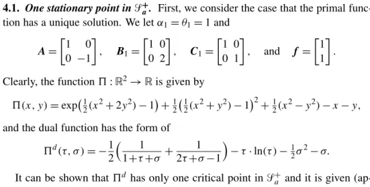
4.1. One stationary point inS+_a. First, we consider the case that the primal func-tion has a unique solufunc-tion. We letα1=θ1=1 and

A= 1 0 0 −1 , B1= 1 0 0 2 , C1= 1 0 0 1 , and f = 1 1 .

Clearly, the function5:_R2→_Ris given by

5(x,y)=_exp 1 2(x 2_+2y2₎₋₁ +1 2 1 2(x 2_+y2₎₋₁2 +1 2(x 2_−y2_)−x−y, and the dual function has the form of

5d_{(τ, σ)= −}1 2 ₁ 1+τ+σ + 1 2τ+σ−1 −τ·_ln(τ)−1 2σ 2_−σ.

It can be shown that5d has only one critical point inS+_a and it is given (ap-proximately) by ς=(₁._{171057661103504},−₀._{34599084656216}). 5.6 5.2 4.8 4.4 4 3.6 3.2 2.8 2.4 2 1.6 1.2 0.8 0.4 0 -0.4 -2 -1.5 -1 -0.5 0 0.5 1 1.5 2 -2 -1.5 -1 -0.5 0 0.5 1 1.5 2 5.6 5.2 4.8 4.4 4 3.6 3.2 2.8 2.4 2 1.6 1.2 0.8 0.4 0 -0.4 -2 _-1.5 -1 _-0.5 0 _0.5 1 _1.5 2 -2-1.5 -1-0.5 00.5 11.5 2 -10 -5 0 5 10

-0.73 -0.84 -0.95 -1.06 -1.17 -1.28 -1.39 -1.5 -1.61 -1.72 -1.83 -1.94 -2.05 -2.16 -2.27 0.5 1 1.5 2 2.5 -1 -0.5 0 0.5 1 1.5 2 -0.73 -0.84 -0.95 -1.06 -1.17 -1.28 -1.39 -1.5 -1.61 -1.72 -1.83 -1.94 -2.05 -2.16 -2.27 0.5 1 1.5 2 2.5 -1-0.5 0 0.5 1 1.5 2 -10 -8 -6 -4 -2 0

Figure 2. Contours and graph of the dual function5d ofSection 4.1. By the triality theory, the vector

x=_G(ς)−1_f =(₀._{54792514555217},₁._{003890602479819}) is the only global minimizer of the primal problem.

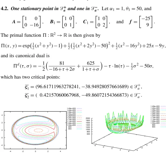
4.2. One stationary point inS+

a and one inS−a. Letα1=1,θ1=50, and

A= 1 0 0 −₁₆ , B1= 1 0 0 1 , C1= 1 0 0 2 , and f = −₂₅ 9 .

The primal function5:_R2→_{Ris then given by}

5(x,y)=_exp 1 2(x 2_+y2₎₋₁ +1 2 1 2(x 2_+2y2₎₋₅₀2₊1 2(x 2_−16y2_)+25x−9y, and its canonical dual is

5d_{(τ, σ)= −}1 2 ₈₁ −16+τ+2σ + 625 1+τ+σ −τ·_ln(τ)−1 2σ 2_−50σ, which has two critical points:

ς₁=(96.61711963278241,−38.94928057661689)∈S+_a, ς2=( 0.42157060067968,−49.86072154366873)∈S − a. 1.49e+003 1.44e+003 1.39e+003 1.34e+003 1.29e+003 1.24e+003 1.19e+003 1.14e+003 1.09e+003 1.04e+003 994 944 -4 -2 0 2 4 -4 -2 0 2 4 1.49e+003 1.44e+003 1.39e+003 1.34e+003 1.29e+003 1.24e+003 1.19e+003 1.14e+003 1.09e+003 1.04e+003 994 944 -4 -2 ₀ 2 4 -4 -2 0 2 4 600 800 1000 1200 1400 1600 1800 2000

720 700 680 660 640 620 600 580 560 540 520 80 85 90 95 100 105 110 -50 -45 -40 -35 -30 -25 720 700 680 660 640 620 600 580 560 540 520 80 ₈₅ 90 ₉₅ 100 ₁₀₅ 110-50 -45 -40 -35 -30 -25 500 550 600 650 700 1.26e+003 1.25e+003 1.25e+003 1.25e+003 1.25e+003 1.25e+003 1.24e+003 1.24e+003 1.24e+003 1 2 3 4 5 6 7 8 9 10-60 -55 -50 -45 -40 1160 1180 1200 1220 1240 1260 1.26e+003 1.25e+003 1.25e+003 1.25e+003 1.25e+003 1.25e+003 1.24e+003 1.24e+003 1.24e+003 1 2 3 4 5 6 7 8 9 10-60 -55 -50 -45 -40 1160 1180 1200 1220 1240 1260

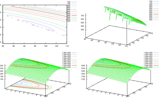
Figure 4. Contours and graph of the dual function5d ofSection 4.2

inS+a (top) and inS

−

a (bottom).

Therefore, by the triality theory, the associated vector

x1=G(ς₁)−1f =(−0.42612784793499,3.310578038951848) is the only global minimizer of5(x), and

x2=(0.51611144112381,−0.078057328303129)

is a local maximizer (seeFigure 3) sinceς₂is a local maximum of5d inS−a (see

Figure 4, bottom).

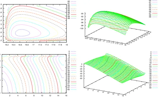
4.3. One stationary point inS+_a and two inS−_a. In order to illustrate the triality theory, we letα1=θ1=2 and

A= −_{16 0} 0 −₄ , B1= 1 0 0 0 , C1= 0 0 0 1 , and f = 2 2 . Accordingly, we have 5(x,y)=_exp 1 2x 2₋₂ +1 2 1 2y 2₋₂2 +1 2(−16x 2_−4y2_)−2x−2y, 5d_{(τ, σ)= −}1 2 ₄ σ−₄+ 4 τ−16 −τ·_ln(τ)−τ−1 2σ 2_−2σ.

In this case,5d has in total six critical points but only one inS+a,

ς1=(16.64468576727409,4.552474610531074)∈S +

0 -5 -10 -15 -20 -25 -30 -35 -40 -45 -50 -55 -60 -65 -70 -75 -80 -85 -4 -2 0 2 4 -6 -4 -2 0 2 4 6 0 -5 -10 -15 -20 -25 -30 -35 -40 -45 -50 -55 -60 -65 -70 -75 -80 -85 -4 -2 ₀ 2 4 -6 -4 -2 0 2 4 6 -100 -50 0 50 100

Figure 5. Contours and graph of the primal function5ofSection 4.3.

(seeFigure 6, top), and two inS−

a:

ς₂=(₀._{13641513779858},−₁._{943380912562619})∈S−_a,

ς₃=(₁₅._{34981976568548},₃._{390906302031545})∈S−_a.

FromFigure 6, bottom, we can see thatς₂is a local maximizer andς₃is a local minimizer of5d_{. Therefore, by the triality theory, we know that}

x1=G(ς1) −1_{f =(3.102286573591542,3.620075858467906)} -90 -91 -92 -93 -94 -95 -96 -97 -98 -99 16.2 16.4 16.6 16.8 17 17.2 17.4 17.6 17.8 18 4.2 4.4 4.6 4.8 5 5.2 5.4 5.6 5.8 6 -90 -91 -92 -93 -94 -95 -96 -97 -98 -99 16.2 16.4 16.6 16.8 17 17.2 17.4 17.6 17.8184.24.4 4.64.85 5.25.4 5.65.86 -100 -98 -96 -94 -92 -90 0 -3 -6 -9 -12 -15 -18 -21 -24 -27 -30 -33 -36 -39 -42 -45 -48 -51 -54 -57 -60 2 4 6 8 10 12 14 16 -2 -1 0 1 2 3 4 -30 -6 -9 -12 -15 -18 -21 -24 -27 -30 -33 -36 -39 -42 -45 -48 -51 -54 -57 -60 2 ₄ 6 ₈ 10 ₁₂ 14 _{16 -2} -1 0 1 2 3 4 -60 -50 -40 -30 -20 -10 0

Figure 6. Contours and graph of the dual function5d ofSection 4.3

is the only global minimizer,

x2=(−0.12607490787063,−0.33650880356205) is a local maximizer, and

x3=(−3.076070133243102,−3.283567054905852) is a local minimizer of5(x)(seeFigure 5).

4.4. Nonunique global minima. In the case that no stationary point can be found inS+_a, the primal problem could have more than one global minima. To see this, we let f ≡_0,α₁=θ₁=_{2, and} A≡₀, _B1= 1 0 0 0 , and C1= 0 0 0 1 .

In this case, the primal function

5(x,y)=_exp 1 2x 2₋₂ +1 2 1 2y 2₋₂2

has two global minimums at(0,−₂) _and(₀,₂) _{and a local maximum at} (₀,₀)_. While the dual function

5d_{(τ, σ)= −τ}

lnτ−τ−1 2σ

2_−2σ does not have a stationary point inS+

a. There is however a critical point in the boundary ofS+

a, namelyς=(exp(−2),0). By definingx=G(ς)

−1_{f, we have} thatx=(₀,₀)_.

In order to find a global minimum of5, we need to introduce the perturbations

An= " −16 n 0 0 −4 n # and fn= "₂ n 2 n # for everyn∈N. Then the associated primal and dual functions are

5n(x,y)=exp 1₂x2−2 +1 2 1 2y 2₋₂2₊1 2 − 16 nx 2₋4 ny 2 −2 nx− 2 ny, 5d n(τ, σ)= − 1 2 4 n2 τ₋16 n + 4 n2 σ₋4 n −τ_lnτ+τ−1 2σ 2_{−2τ−2σ.}

Notice that ifn=_{1 we are in the case presented inSection 4.3. Let us show that for} sufficiently large values ofnwe can find a stationary point for5d_n inS+_a, namelyς_n. Furthermore, by definingxn=_G(ς_n)−1_{fn, we will have a convergent sequence.}

Let us calculate the gradient of5dn:

∇5d_n(τ, σ)= " −₂−_lnτ+ 2 (nτ−16)2 −σ−₂+ 2 (nσ−4)2 # .

Leth(τ)= −₂−_lnτ+₂/(nτ−₁₆)2_andg(σ)= −σ−₂+₂/(nσ−₄)2_{. It is} not difficult to show that there exists a sufficiently large N∈_{Nsuch that, if}n>N,

•_n·_exp −₂+1 n

−_{16 and}n·_exp(−₂)−_{16 are positive numbers},

•_{h exp} −₂+1 n = 2 n·_exp −₂+1 n −₁₆2 −1 n<0<h(exp(−2)) = 2 (n·_exp(−₂)−₁₆)2, •_g 5.1 n ≈ −5.1 n −0.34710743801<0<g 4.9 n ≈0.46913580247−4.9 n .

Based on these results, we know that, for every n > N, ∇5d_n has a station-ary pointς_n =(τ_n, σ_n)∈ _exp(−₂),_exp −₂+1

n ×4.9 n , 5.1 n . Moreover, since g(σn)=0, it is easy to obtain lim

n→+∞n

·σ_n=_5. Notice also that

G(ςn)=

τn−16_n 0 0 σn−4_n

is positive definite. Therefore, the perturbed solution can be obtained as xn=G(ςn) −1_fn= " 2/(n·τ_n−₁₆) 2/(n·σ_n−₄) # . Sinceτn∈ exp(−₂),_exp −₂+1 n , we have lim n→+∞τn

=_exp(−₂)_{. From the fact} that lim n→+∞n ·σ_n=_{5, we get} lim n→+∞xn = 0 2 , which is a solution of5.

Canonical perturbation method was originally introduced in[Ruan et al. 2010]

for solving nonconvex polynomial minimization problems. This method has been used successfully in integer programming and network communication (see[Gao et al. 2012;Wang et al. 2012]).

5. Future research

Some open questions that will be studied in the future are the following:

• _{As stated inRemark 1, in order to use the canonical dual transformation, a}

neces-sary condition is that(P)has a unique solution. Is this also a sufficient condition? In other words, given(P)such that it has a unique solution, can we find a stationary point of5d inS+_a?

• _{Section 4.4 shows an interesting perturbation method that allows us to solve}

a problem when the necessary condition ofRemark 1 is not satisfied. Can we generalize this method and develop an algorithm?

Appendix A: Some lemmas in matrix analysis The following results are needed in the proofs ofSection 2:

Lemma A1(singular-value decomposition [Horn and Johnson 1985]). For any given matrix M⊂_Rm×n withRank(M)=r,there existU ⊂_Rm×m, R⊂_Rm×n, andE⊂_Rn×nsuch that

M=UR E,

whereUandEare orthogonal matrices,and Ri j =

si if i= j and i=1, . . . ,r, 0 if i6= j,

where si >0for every i=1, . . . ,r .

Lemma A2[Horn and Johnson 1985]. IfGandU are positive-definite matrices inRn×n,thenG_Uif and only ifU−1_G−1.

Lemma A3[Gao and Wu 2012]. Suppose P,U,and Dare three matrices inRn×n

such that D= D11 0m×(n−m) 0₍n−m)×n 0(n−m)×(n−m) ,

where D11∈Rm×mis nonsingular and

P= P11 P12 P21 P22 ≺₀ and U= U11 0m×(n−m) 0₍n−m)×m U22 ₀, where Pi j andUi i are appropriate-dimensional matrices for i, j=₁,_{2. Then}

P+DU Dt 0 ⇐⇒ −DtP−1D−U−10. Acknowledgements

This research is supported by the US Air Force Office of Scientific Research under the grant AFOSR FA9550-10-1-0487. Comments and suggestions from the editor and reviewers are sincerely acknowledged.

References

[Aspnes et al. 2004] J. Aspnes, D. Goldberg, and Y. R. Yang,“On the computational complexity

of sensor network localization”, pp. 32–44 inAlgorithmic aspects of wireless sensor networks

(Turku, 2004), edited by S. Nikoletseas and J. D. P. Rolim, Lecture Notes in Computer Science

3121, Springer, Berlin, 2004.

[Cai et al. 2014] K. Cai, D. Y. Gao, and Q. H. Qin,“Post-buckling solutions of hyper-elastic beam by

canonical dual finite element method”,Math. Mech. Solids19:6 (2014), 659–671. arXiv 1302.4136

[Desoer and Whalen 1963] C. A. Desoer and B. H. Whalen,“A note on pseudoinverses”,J. Soc.

[Feng et al. 2012] J.-M. Feng, G.-X. Lin, R.-L. Sheu, and Y. Xia,“Duality and solutions for quadratic programming over single non-homogeneous quadratic constraint”,J. Glob. Optim.54:2 (2012), 275–293.

[Gao 1996] D. Y. Gao,“Complementary finite-element method for finite deformation nonsmooth

mechanics”,J. Eng. Math.30:3 (1996), 339–353.

[Gao 1997] D. Y. Gao,“Dual extremum principles in finite deformation theory with applications

to post-buckling analysis of extended nonlinear beam theory”,Appl. Mech. Rev.(ASME)50:11S (1997), S64–S71.

[Gao 1998] D. Y. Gao,“Duality, triality and complementary extremum principles in non-convex

parametric variational problems with applications”,IMA J. Appl. Math.61:3 (1998), 199–235.

[Gao 1999] D. Y. Gao,“General analytic solutions and complementary variational principles for

large deformation nonsmooth mechanics”,Meccanica(Milano)34:3 (1999), 169–198.

[Gao 2000a] D. Y. Gao,“Canonical dual transformation method and generalized triality theory in

nonsmooth global optimizaton”,J. Glob. Optim.17:1-4 (2000), 127–160.

[Gao 2000b] D. Y. Gao,Duality principles in nonconvex systems: theory, methods and applications,

Nonconvex Optimization and its Applications39, Kluwer, Dordrecht, 2000.

[Gao 2003a] D. Y. Gao,“Nonconvex semi-linear problems and canonical duality solutions”, pp.

261–312 inAdvances in mechanics and mathematics, vol. 2, edited by D. Y. Gao and R. W. Ogden,

Adv. Mech. Math.4, Kluwer, Boston, 2003.

[Gao 2003b] D. Y. Gao,“Perfect duality theory and complete solutions to a class of global

optimiza-tion problems”,Optimization52:4-5 (2003), 467–493.

[Gao 2009] D. Y. Gao,“Canonical duality theory: theory, method, and applications in global

opti-mization”,Comput. Chem. Eng.33:12 (2009), 1964–1972.

[Gao and Ogden 2008a] D. Y. Gao and R. W. Ogden,“Multiple solutions to non-convex variational

problems with implications for phase transitions and numerical computation”,Quart. J. Mech. Appl. Math.61:4 (2008), 496–522.

[Gao and Ogden 2008b] D. Y. Gao and R. W. Ogden,“Closed-form solutions, extremality and

non-smoothness criteria in a large deformation elasticity problem”,Z. Angew. Math. Phys.59:3 (2008), 498–517.

[Gao and Ruan 2008] D. Y. Gao and N. Ruan,“Solutions and optimality criteria for nonconvex

quadratic-exponential minimization problem”,Math. Methods Oper. Res.67:3 (2008), 479–491.

[Gao and Sherali 2009] D. Y. Gao and H. D. Sherali,“Canonical duality theory: connections

be-tween nonconvex mechanics and global optimization”, pp. 257–326 inAdvances in applied math-ematics and global optimization, edited by D. Y. Gao and H. D. Sherali, Adv. Mech. Math.17, Springer, New York, 2009.

[Gao and Strang 1989] D. Y. Gao and G. Strang, “Geometric nonlinearity: potential energy,

comple-mentary energy, and the gap function”,Quart. Appl. Math.47:3 (1989), 487–504.

[Gao and Wu 2012] D. Y. Gao and C. Wu,“On the triality theory for a quartic polynomial

optimiza-tion problem”,J. Ind. Manag. Optim.8:1 (2012), 229–242.

[Gao and Yu 2008] D. Y. Gao and H. Yu,“Multi-scale modelling and canonical dual finite element

method in phase transitions of solids”,Int. J. Solids Struct.45:13 (2008), 3660–3673.

[Gao et al. 2012] D. Y. Gao, N. Ruan, and P. M. Pardalos,“Canonical dual solutions to sum of

pp. 37–54 inSensors: theory, algorithms, and applications, edited by V. L. Boginski et al., Springer

Optim. Appl.61, Springer, New York, 2012.

[Horn and Johnson 1985] R. A. Horn and C. R. Johnson,Matrix analysis, Cambridge University

Press, 1985.

[Marsden and Hughes 1983] J. E. Marsden and T. J. R. Hughes,Mathematical foundations of

elas-ticity, Prentice-Hall, Englewood Cliffs, NJ, 1983.

[MAXIMA 2010] MAXIMA,“Maxima, a computer algebra system”, 2010, Available at http://

maxima.sourceforge.net. Version 5.22.1.

[Moré and Wu 1997] J. J. Moré and Z. Wu,“Global continuation for distance geometry problems”,

SIAM J. Optim.7:3 (1997), 814–836.

[Moreau 1968] J.-J. Moreau, “La notion de sur-potentiel et les liaisons unilatérales en

élastosta-tique”,C. R. Acad. Sci. Paris Sér. A-B267A(1968), A954–A957.

[Moreau et al. 1988] J.-J. Moreau, P. D. Panagiotopoulos, and G. Strang (editors),Topics in

non-smooth mechanics, Birkhäuser, Basel, 1988.

[Peters and Wilkinson 1970] G. Peters and J. H. Wilkinson,“The least squares problem and

pseudo-inverses”,Comput. J.13:3 (1970), 309–316.

[Ruan and Gao 2014a] N. Ruan and D. Y. Gao,“Canonical duality approach for non-linear

dynami-cal systems”,IMA J. Appl. Math.79:2 (2014), 313–325.

[Ruan and Gao 2014b] N. Ruan and D. Y. Gao,“Global optimal solutions to a general sensor network

localization problem”,Perform. Eval.75–76(2014), 1–16.

[Ruan et al. 2010] N. Ruan, D. Y. Gao, and Y. Jiao,“Canonical dual least square method for solving

general nonlinear systems of quadratic equations”,Comput. Optim. Appl.47:2 (2010), 335–347.

[Santos and Gao 2012] H. A. F. A. Santos and D. Y. Gao,“Canonical dual finite element method for

solving post-buckling problems of a large deformation elastic beam”,Int. J. Nonlinear Mech.47:2 (2012), 240–247.

[Saxe 1979] J. B. Saxe, “Embeddability of weighted graphs in k-space is strongly NP-hard”, pp. 480–

489 inProceedings of the 17th Allerton Conference on Communications, Control, and Computing

(Monticello, IL, 1979), University of Illinois at Urbana-Champaign, Urbana, IL, 1979. Also inTwo

papers on graph embedding problems, preprint, Carnegie Mellon University, Pittsburgh, PA, 1980.

[Strugariu et al. 2011] R. Strugariu, M. D. Voisei, and C. Z˘alinescu,“Counter-examples in bi-duality,

triality and tri-duality”,Discrete Contin. Dyn. Syst.31:4 (2011), 1453–1468.

[Voisei and Z˘alinescu 2011] M. D. Voisei and C. Z˘alinescu,“Some remarks concerning Gao–Strang’s

complementary gap function”,Appl. Anal.90:6 (2011), 1111–1121.

[Wang et al. 2012] Z. Wang, S.-C. Fang, D. Y. Gao, and W. Xing,“Canonical dual approach to

solving the maximum cut problem”,J. Glob. Optim.54:2 (2012), 341–351.

[Xie and Schlick 2000] D. Xie and T. Schlick,“Visualization of chemical databases using the

sin-gular value decomposition and truncated-Newton minimization”, pp. 267–286 inOptimization in computational chemistry and molecular biology: local and global approaches, edited by C. A.

Floudas and P. M. Pardalos, Optimization in Computational Chemistry and Molecular Biology40,

Springer, Dordrecht, 2000.

[Zhang et al. 2011] J. Zhang, D. Y. Gao, and J. Yearwood,“A novel canonical dual computational

approach for prion AGAAAAGA amyloid fibril molecular modeling”,J. Theoret. Biol.284(2011), 149–157.

Received 22 Apr 2013. Revised 13 May 2014. Accepted 29 Jul 2014. DANIELMORALES-SILVA: [email protected]

School of Science, Information Technology and Engineering, Federation University, Mt. Helen VIC 3353, Australia

DAVIDY. GAO: [email protected] [email protected]

School of Science, Information Technology and Engineering, Federation University, Mt. Helen, VIC 3353, Australia

and

Research School of Engineering, Australian National University, Canberra, ACT 0200, Australia

M M∩