Optimized Crossover Genetic Algorithm to Minimize the Maximum Lateness of Single Machine Family Scheduling Problems
Habibeh Nazif (Department of Mathematics, Payame Noor University,I. R of Iran)
Lee Lai Soon (Department of Mathematics, Universiti Putra Malaysia, 43400 UPM Serdang, Selangor, Malaysia)
240 Author (s)
Habibeh Nazif,
Department of Mathematics, Payame Noor University, I. R of Iran
E-mail:[email protected],
Lee Lai Soon
Department of Mathematics, Universiti Putra Malaysia, 43400 UPM Serdang, Selangor, Malaysia
E-mail:[email protected]
Optimized Crossover Genetic Algorithm to Minimize the Maximum Lateness of Single Machine Family Scheduling Problems
Abstract
We address a single machine family scheduling problem where jobs are partitioned into families and setup time is required between these families. For this problem, we propose a genetic algorithm using an optimized crossover operator to find an optimal schedule which minimizes the maximum lateness of the jobs in the presence of the sequence independent family setup times. The proposed algorithm using an undirected bipartite graph finds the best offspring solution among an exponentially large number of potential offspring. Extensive computational experiments are conducted to assess the efficiency of the proposed algorithm compared to other variants of local search methods namely dynamic length tabu search, randomized steepest descent method, and other variants of genetic algorithms. The computational results indicate the proposed algorithm is generating better quality solutions compared to other local search algorithms.
Keywords: Genetic Algorithm, Single Machine Scheduling, Maximum Lateness Introduction
Machine Scheduling Problems (MSPs) are one of the classical combinatorial optimization problems which exist in many diverse areas such as transportation, manufacturing system, etc. The main focus is on the efficient allocation of one or more resources to activities over time. An excellent survey can be found in (Lawler et al., 1993). A single machine scheduling problem is one where there are N jobs to be scheduled on a single machine. In this paper, we consider a Single Machine Family Scheduling Problem (SMFSP), where jobs are partitioned into families and setup time is required between these families. (Hariri and Potts, 1997) describe the problem in which N jobs, each characterized by a processing time 𝑝𝑗 and a due date 𝑑𝑗,
for 𝑗 = 1,2, … , 𝑁, are partitioned into F families. For each family f (𝑓 = 1, 2, … , 𝐹), jobs are split into batches, where a batch is defined as a maximal set of contiguously scheduled jobs from the same family which share the same setup time. A sequence
independent family setup time 𝑠𝑓, is required
at the start of the schedule and also whenever there is a switch in processing jobs from one family to jobs of another family. We assume that all the jobs are available at time zero. The objective is to find a schedule which minimizes the maximum lateness 𝐿𝑚𝑎𝑥 of the jobs. The
SMFSP for arbitrary family f is an NP-hard problem as shown by (Bruno and Downey, 1978). This problem can be represented as 1|𝑠𝑓| 𝐿𝑚𝑎𝑥 based on the standard
classification of (Graham et al., 1979).
241 (OCGA) for the problem of 1|𝑠𝑓| 𝐿𝑚𝑎𝑥. The
objective is to find a schedule which minimizes the maximum lateness 𝐿𝑚𝑎𝑥 of
the jobs in the presence of the sequence independent family setup times 𝑠𝑓.
Literature Review
Numerous optimization methods including exact methods, heuristics and local search algorithms have been proposed for the problem of 1|𝑠𝑓| 𝐿𝑚𝑎𝑥. Excellent reviews on
scheduling with setup considerations are given by (Potts and Kovalyov, 2000) and (Allahverdi et al., 1999, 2008).
(Monma and Potts, 1989) show that there exists an optimal schedule in which the Earliest Due Date (EDD) rule of (Jackson, 1955) applies within each family f. They consider a variety of SMFSPs under the assumption that the `triangle inequality' holds for each machine i, which means that 𝑠𝑖𝑓≤ 𝑠𝑖𝑓𝑔+𝑠𝑖𝑔 , for all distinct families f,
g and h. Using dynamic programming, they solve the problems of 1|𝑠𝑓𝑔| 𝐿𝑚𝑎𝑥 and
1|𝑠𝑓| 𝐿𝑚𝑎𝑥 in 𝑂(𝐹2𝑁𝐹
2+2𝐹
) and 𝑂(𝐹2𝑁2𝐹)
time respectively. (Hariri and Potts, 1997) propose a branch and bound (B&B) algorithm for the problem of 1|𝑠𝑓| 𝐿𝑚𝑎𝑥.
They obtained an initial lower bound by ignoring setups, except for those associated with the first job in each family, and solved the resulting problem with the EDD rule. This lower bound is improved by a procedure that considers whether or not certain families are split into two or more batches. Computational results show that the algorithm is successful in solving instances for up to about 50 jobs.
(Baker and Magazine, 2000) design an algorithm that uses a B&B approach combined with dominance properties which reduced the effective problem size to solve the problem of 1|𝑠| 𝐿𝑚𝑎𝑥, where setup times
are identical. The identification of composite jobs allows the effective problem size to be reduced before the enumeration begins. Their proposed algorithm solves problems with up to 60 jobs.(Zdrzałka, 1991) develops
heuristic methods for 1|𝑠𝑓| 𝐿𝑚𝑎𝑥 in which
there are unit setup times, and under the assumption that due dates are non-positive to ensure that the objective function is positive. When all jobs of family are scheduled contiguously, computational results are shown to have a maximum lateness which does not exceed twice the optimal value. Moreover (Zdrzałka, 1995) proposes two approximation algorithms without the unit setup time assumption and under non-positive due dates. The algorithm starts with a schedule in which each batch contains all jobs from a family, and allows each family to be split into at most two batches. The algorithm requires 𝑂(𝑁2) time
and it generates a schedule with maximum lateness that is no more than 3/2 times the optimal value.
(Hariri and Potts, 1997) design two heuristics in which the first heuristic assigns all jobs of a family to a single batch, and the second heuristic splits each family into at most two batches according to the due dates of its jobs. They show that both heuristics require O(N log N) time. They also show that the first heuristic has a worst case performance ratio of 2-1/F, where a composite heuristic algorithm which selects the better of the schedules generated by the two heuristic has a worst case analysis of 5/3 for arbitrary F. (Pan et al., 2001) suggest a mathematical model that first finds an initial schedule and then applies merging properties to improve the initial schedule. Computational results show that their algorithm is successful in solving problems with up to 1000 jobs. (Schultz et al., 20004) develop a new neighborhood search heuristic for solving problem 1|𝑠𝑓| 𝐿𝑚𝑎𝑥
based on the properties and theorems presented by (Hariri and Potts, 1997) and (Baker, 1999). The procedure is computationally efficient for problem instances with 500 jobs.
242 set up times. When a machine processes two
jobs from the same family one after the other, no set-up time is required. Extensive computational experiments where test problems are randomly generated, show that the rolling horizon procedure outperforms other heuristic algorithms except when setup factors are large.
(Jin et al., 2009) propose a batch-based simulated annealing algorithm (BSA) with the new neighborhood developed based on batch destruction and construction. Experiments are carried out on the randomly generated problems and the real-life instances from a factory. Computational results show that the proposed algorithm outperforms the standard simulated annealing (SSA) in both solution quality and computational effort. Algorithm BSA also outperforms the existing RH algorithm. Results of the real-life problems also show that BSA algorithm can obtain near optimal solutions in 0.1 s.
(Lee et al., 2007) propose a MultiCrossover Genetic Algorithm (MXGA) for the problem of 1|𝑠𝑓| 𝐿𝑚𝑎𝑥. They hypothesize that
generating multiple offspring during the crossover can improve the performance of a genetic algorithm. Computational experiments of 50 and 100 jobs show that the proposed MXGA achieves better solutions compared to a standard genetic algorithm, both standard and dynamic length tabu search and a randomized steepest descent method.
Optimized Crossover Genetic Algorithm (OCGA)
Genetic Algorithms (GAs) were first proposed by (John Holland, 1975). The GA is a heuristic search technique that simulates the processes of natural selection and evolution. A GA maintains a population of individuals over many generations. An initial population of individuals, each representing a feasible solution to the given problem is constructed at random. For each generation, the fitness value of each individual in the population is measured, where a high fitness value would exhibit a
better solution compared to a low fitness value. Fitter members are more likely to be selected from the population using a selection mechanism to produce offspring for the subsequent generation via crossover and mutation. After many generations the result is hopefully a population that is substantially fitter than the original.
Most of the crossover mechanisms determine offspring using a stochastic approach and without reference to the objective function. (Aggarwal et al., 1997) propose an optimized crossover mechanism for the independent set problem which takes into account the objective function in a straightforward way. They recognize that the merge operation formulated by (Balas and Niehaus, 1996) can be thought of as an optimized crossover. Hence, they construct a bipartite graph from the two parent independent sets and determine an optimum child using a matching algorithm in the graph.
Moreover, they consider the parent which is least similar to the optimum child as the second child. (Balas and Niehaus, 1998) develop this approach to produce a superior genetic algorithm. They examine variations of each element of the genetic algorithm and develop a steady state replacement that performs better than its competitors on most problems. (Ahuja et al., 2000) propose a greedy genetic algorithm which uses two crossover schemes called path crossover and optimized crossover for the quadratic assignment problem. The results on a large set of standard problems show that path crossover performs slightly better than optimized crossover.
243 within the population a binary mutation is
randomly applied to each child. Moreover elitism replacement scheme and filtration strategy are used to preserve good solutions and to avoid premature convergence. The general framework of OCGA can be shown as follows:
Algorithm OCGA begin
Initialize Population (randomly generated); Fitness Evaluation;
repeat
Selection (probabilistic binary tournament selection);
Optimized Crossover;
F-point Swap (if the optimized crossover is not applied);
Mutation (binary mutation); Fitness Evaluation;
Elitism replacement with Filtration; until the end condition is satisfied; return the fittest solution found;
end
Encoding Scheme and Selection Mechanism
A natural way of coding the problem would be to represent each solution by a bit string. We use a binary {0, 1} representation that (Mason, 1992) applied for solving the problem of 1|𝑠𝑓| 𝑤𝑗𝐶𝑗. Using this binary
representation we defined the partition of families into batches, where `1' means the first job in a batch and `0' means a contiguously sequenced job in a batch. The length of the individual corresponds to the number of jobs N. After choosing the representation, we uniformly randomly generate an initial population which is of size 100 in our implementation using a random number generator. We assume that the size of population is kept constant throughout the process.
Moreover we use a probabilistic binary tournament selection scheme to select individuals from the population to be the parents for the OCGA with a given selection probability 𝑝𝑠 = 0.75 based on initial
investigation presented in section computational experiments. In other words, we give a 75% chance for the fitter individual to be selected as the parent
compared to the less fit individual which only has a 25% chance to be selected.
Fitness Evaluation
The fitness function is used to evaluate the individuals which are introduced into the population. We can define the fitness function using the property of EDD rule for batches developed by (Baker, 1999), in which there exists an optimal schedule where the batches are sequenced in a non-decreasing order according to their due dates. As mentioned earlier, a batch is a maximum group of contiguously scheduled jobs within a family. Let 𝑑𝑓𝑗 and 𝑝𝑓𝑗 denote
the due date and processing time of the jth job from family f which is identified as pair (f, j). Let (f, h) ,..., (f, k) be the jobs of an arbitrary batch b, then the batch due date 𝛿𝑏is defined as follows:
𝛿𝑏= min
j=h,…,k 𝑑𝑓𝑗+ 𝑞𝑓𝑗 where 𝑞𝑓𝑗 = 𝑝𝑓𝑖 𝑘
𝑖=
− (𝑝𝑓+ ⋯ + 𝑝𝑓𝑗)
In an optimal schedule, the batches are sequenced in a non-decreasing order according to their batch due dates 𝛿𝑏(i. e. 𝛿𝑏≤ 𝛿𝑏+1). A sequence independent
family setup time 𝑠𝑓 is added before the start
of each batch and when there is a switch in the processing jobs from one family to jobs of another family. We define fitness function as the maximum lateness 𝐿𝑚𝑎𝑥 of
the schedule defined as 𝐿𝑚𝑎𝑥 = max j {𝐿𝑗}
where 𝐿𝑗 = 𝐶𝑗− 𝑑𝑗 and 𝐶𝑗 denotes the
completion time of job j.
Optimized Crossover
244 the search space. We will now explain the
optimized crossover strategy on determining O-child and E-child for the problem of 1|𝑠𝑓| 𝐿𝑚𝑎𝑥.
Step 1:
Identify the parent with the least 𝐿𝑚𝑎𝑥 as 𝑃1 and select thefamily within the 𝑃1,which contains
the job where 𝐿𝑚𝑎𝑥 occurs as
family f. Label another parent as 𝑃2. Note that this family f will
be used in both 𝑃1 and 𝑃2.
Step 2:
Construct an undirected bipartite graph 𝐺 = 𝑈 ∪ 𝑉, 𝐸 where𝑈 = {𝑢1, 𝑢2 , … , 𝑢𝑛 } representing
the jobs of family f, 𝑉 =
{𝑣1, 𝑣1′, 𝑣2 ,𝑣2′,…, 𝑣𝑛 ,𝑣𝑛 ′}
representing bit situation of the jobs of family f in both 𝑃1 and
𝑃2 (i. e. 𝑣𝑖 , 𝑣𝑖 ′ ∈ {1,0}), and E
representing the arc set in the graph in which, {𝑢𝑗, 𝑣𝑖 }, 𝑢𝑗 , 𝑣𝑖 ′ ∈ 𝐸 if
and only if jobs j is represented with the bit situation 𝑣𝑖 and
𝑣𝑖′respectively.
Step 3:
Determine all the maximum matchings in graph G. Suppose that there are k jobs in family f that are represented with a different bit situation in the two parents. There will be exactly 2𝑘maximummatchings in graph G.
Step 4:
Generate a temporary offspring from 𝑃1 by replacing the bitsituation
s of the jobs in family f which corresponds to one of the maximum matchings in graph G. Repeat the procedure for 2𝑘−
1 times to generate 2𝑘temporary
offspring. Note that one of the temporary offspring is exactly the same as 𝑃1 , so we remove it.
Step 5:
Select a temporary offspring with the least 𝐿𝑚𝑎𝑥 among 2𝑘−1 temporary offspring as O-child.
Step 6:
Generate E-child from 𝑃2byreplacing the bit situations of the jobs in family f with ((𝑓𝑝1∪
𝑓𝑝2 )\𝑓𝑂−𝑐𝑖𝑙𝑑 ) ∪ (𝑓𝑝1 ∩ 𝑓𝑝2 ), where 𝑓𝑖 indicates family f of
individual i.
Since the number of temporary offspring will increase exponentially with the number k, we restricted the maximum temporary offspring in graph G in every case to 25
even if the jobs that have a different bit situation in two parents are more than 5. In addition the proposed optimized crossover is applied based on a crossover probability, 𝑝𝑐 = 0.75. In other words, the proposed
optimized crossover is applied to 75% of pairs of selected parents. We demonstrate the proposed optimized crossover by an example as in Figure 1.
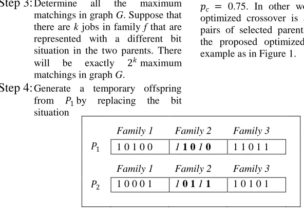
Figure 1: Two parent 𝑃1 and 𝑃2
Given the two parents 𝑃1 and 𝑃2with 15
jobs that are partitioned into 3 families. Suppose that 𝑃1 has the least 𝐿𝑚𝑎𝑥 which
occurs in job 3 of family 2. We formulate an undirected bipartite graph G of the jobs of Family 1 Family 2 Family 3
𝑃1 1 0 1 0 0 1 1 0 1 0 1 1 0 1 1
Family 1 Family 2 Family 3
245 family 2 in both 𝑃1 and 𝑃2 that is shown in Figure 2.
𝑢1= job 1 𝑢2= job 2 𝑢3= job 3 𝑢4= job 4 𝑢5= job 5
𝑣1= 𝑣1′ = 1 𝑣2= 1 𝑣2′ = 0 𝑣3= 0 𝑣3′ = 1 𝑣4= 𝑣4′ = 1 𝑣5= 0 𝑣5′ = 1
Figure 2: Undirected bipartite graph G of the jobs of family 2 in both 𝑃1 and 𝑃2
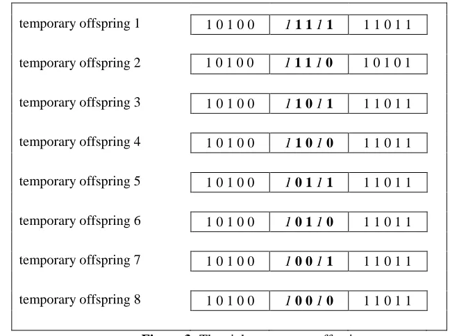
In this case, the jobs 2, 3, and 5 of family 2 are represented with a different bit situation in both 𝑃1 and 𝑃2 , so k = 3 and we can
obtain 23 maximum matchings in this graph.
The eight temporary offspring constructed by replacing the bit situations of the jobs in
family 2, corresponds to each maximum matchings, are shown in Figure 3
Figure 3: The eight temporary offspring Note that the fourth temporary offspring is
the same as 𝑃1 , so we remove it. Suppose
that the seventh temporary offspring has the least 𝐿𝑚𝑎𝑥, then we select it as O-child and
we generate
the E-child from 𝑃2 using Step 6. The
O-child and E-O-child are shown in Figure4.
Figure 4: The O-child and E-child
temporary offspring 1 1 0 1 0 0 1 1 1 1 1 1 1 0 1 1
temporary offspring 2 1 0 1 0 0 1 1 1 1 0 1 0 1 0 1
temporary offspring 3 1 0 1 0 0 1 1 0 1 1 1 1 0 1 1
temporary offspring 4 1 0 1 0 0 1 1 0 1 0 1 1 0 1 1
temporary offspring 5 1 0 1 0 0 1 0 1 11 1 1 0 1 1
temporary offspring 6 1 0 1 0 0 10 1 10 1 1 0 1 1
temporary offspring 7 1 0 1 0 0 1 0 0 1 1 1 1 0 1 1
temporary offspring 8 1 0 1 0 0 10 0 1 0 1 1 0 1 1
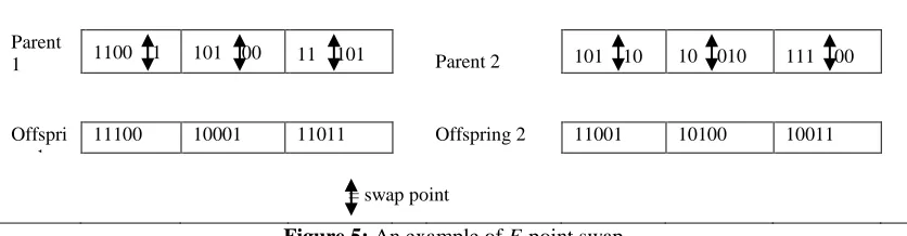
246 F-point Swap:eproduction of parents is
used when crossover operator is not applied to the selected parents in a standard GA. (Lee et al., 2007) use a swap operator instead of the exact duplicate of the parents in their MXGA. In our study, we use a F-point swap operator to produce two new offspring when the optimized crossover is not applied to the parents. This operator could be regarded as a giant mutation where the elements in the parent are randomly reassigned. The process of F-point swap operator is as follows:
Step 1:
Select randomly a swap point within family f = 1 from a parent to form two sub-strings.Step 2:
Swap the position of the sub-strings (except the first job in the selected family) with the swap point as thepoint of exchange.
Step 3:
Repeat Step 1 and Step 2 for each family f (𝑓 = 2, 3, … , 𝐹).The steps above are repeated for the second parent to create a second offspring. An example of F-point swap operator for the two parents is given in Figure 5. A swap point is chosen randomly between the fourth gene and the fifth gene from family 1 in parent 1. Two sub-genes ({1,0,0},{1}) are formed in family 1. Note that the first gene in family 1 is not in the list of the sub genes and it will remain unchanged. We swap the sub-genes in family 1 and repeat these steps for other families in parent 1. After completion a new offspring is obtained from parent 1. Similarly, offspring 2 is formed from parent 2.
Figure 5: An example of F-point swap Mutation
We use binary mutation operator in our OCGA. Binary mutation is applied randomly to each offspring individually that alters each gene from `1' to `0' or vice versa with a given mutation probability 𝑝𝑚 = 1/N,
where N is the number of jobs. Note that each gene can be selected to be mutated except the first gene in each family.
When a gene is flipped from `0' to `1', it means we split a single batch into two separated batches. We combine two contiguously scheduled batches into one single batch if the gene is flipped from `1' to `0'. In this case, the total number of the jobs in the new batch equal to the sum of the jobs in the previous two separated batches.
Replacement
In our study, we use elitism replacement scheme where the good individuals will survive for the next generation and are never lost unless better solutions are found. The elitism replacement is applied as follows: both parent and offspring populations are combined into a single population and sorted in a non-increasing order of their associated fitness value. Then, the first half of the combined population is selected as the individuals of the new population for the next generation.
In order to avoid premature convergence and to add diversity to the new population, we use the filtration strategy proposed by (Lee et al., 2007). Identical individuals are identified from the new population and, they
Parent
1 1100 1 101 00 11 101 Parent 2 101 10 10 010 111 00
Offspri ng 1
11100 10001 11011 Offspring 2 11001 10100 10011
247 are removed and replaced by uniformly
randomly generated new individuals. Since a certain amount of computational time is required during the filtration strategy, so we apply the filtration in every 50 generations.
Computational Experiments
In this section, we present the computational results of the proposed OCGA and the comparisons with other variants of local search methods namely Standard Genetic Algorithm (SGA), Dynamic Length Tabu Search (DLTS), Randomized Steepest Descent Method (RSDM), and Multicrossover Genetic Algorithm (MXGA) where the last three algorithms are proposed by (Lee et al., 2007). The algorithms are coded in C language and implemented on a Pentium 4, 2.0 GHz computer with 2.0 GB RAM.
We genarated problem instances with 50 and 100 jobs, and with 4, 8 and 12 families. Jobs are distributed uniformly across families, so that each family contains 𝑁/𝐹 or 𝑁/𝐹 jobs. This classification of problem instances have been widely used by other literature so we adopt it for our computational experiments.
In each problem, processing times are randomly generated integers from an uniform distribution defined on [1, 100]. We also generated five sets of integer due dates from the uniform distribution [0, 𝛼𝑃], where 𝛼 ∈ {0.2, 0.4, 0.6, 0.8, 1.0}, and P is summation of generated processing times in each problem. Based on (Hariri and Potts, 1997), the three setup times class A, B and C are randomly generated integers from the three uniform distributions [1, 100], [1, 20] and [101, 200] respectively. For each combination of N, F, 𝛼 and setup times class, five problem instances are created.
We used the lower bound proposed by algorithms. Algorithms are compared by listing, for each combination of value N, F, 𝛼 and setup times class, the average relative percentage deviation (ARD) and the maximum relative percentage deviation (MRD) of the heuristic solution value from
the lower bound. The ARD and MRD formulas are shown in equations (1) and (2) respectively.
𝐴𝑅𝐷 =
(𝑈𝐵 𝑖𝑟 −𝐿𝐵 𝑖
𝐿𝐵 𝑖 ×100 %) 𝑅
𝑟 =1 𝐼 𝑖=1
𝐼𝑅 (1)
𝑀𝑅𝐷 = max𝑖=1,2,…,𝐼
𝑟=1,2,…,𝑅
(𝑈𝐵𝑖𝑟−𝐿𝐵𝑖
𝐿𝐵𝑖 × 100%) (2)
where,
I= number of problem instances with the relevant combination of parameters;
R= number of repeated runs for problem instance i (𝑖 = 1, 2, … , 𝐼);
𝑈𝐵𝑖𝑟= heuristic solution found in rth run of
problem instance i;
𝐿𝐵𝑖= lower bound of the problem instance i.
Initial Investigations of OCGA
We gradually construct the proposed algorithm from the standard GA. The differences between the OCGA and SGA are with regards to the use of the crossover operator, reproduction procedure and the replacement scheme. For the initial investigation, five problem instances with five combinations of due dates are generated as described earlier and setup time class A is used in this experiment. For each combination of the problem instance and the due date range, a total of 30 runs were performed to obtain the average value. In order to have a fair comparison in this experiment, a fixed time limit of 15 CPU seconds per run is imposed.
In the first investigation, we employ selection probability 𝑝𝑠with four different
values in the SGA to determine the most efficient value of 𝑝𝑠 which will be used in
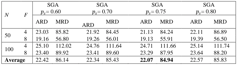
248 Table 1: Comparison among selection probabilities (15 CPU seconds per run)
N F
SGA 𝑝𝑠= 0.60
SGA 𝑝𝑠= 0.70
SGA 𝑝𝑠= 0.75
SGA 𝑝𝑠= 0.80
ARD MRD
ARD MRD ARD MRD ARD MRD
50 4 23.03 85.82 21.92 84.45 21.13 84.24 22.11 86.89 8 19.16 56.80 19.26 56.01 19.13 55.91 19.39 56.50
100 4 25.10 112.02 24.76 111.64 24.71 111.66 25.14 111.74 8 23.40 89.92 23.41 89.60 23.29 87.95 23.64 88.20 Average 22.42 86.14 22.34 85.43 22.07 84.94 22.57 85.83
For each algorithm the entries report the average value of ARD and MRD computed over the five problem instances with five combinations of due dates (i.e. 750 runs) and the final line gives the overall value. It is clear that better solution quality is obtained under the optimized crossover operator. From Table 1, we can conclude that a selection probability of 0.75 can be
effective for getting better results. Table 2 shows the computational results of the optimized crossover operator employed in the SGA compared to the 1-point crossover operator. The results of this investigation determine whether our proposed optimized crossover operator is advantageous to produce offspring during crossover.
Table 2: Comparison between crossover operators (15 CPU seconds per run) N F Optimized Crossover 1-point Crossover
ARD MRD ARD MRD
50 4 18.62 79.00 21.80 83.45
8 17.69 56.40 19.33 61.95
100 4 21.06 99.61 24.92 105.16
8 19.30 84.31 22.18 86.70
Average 19.17 79.83 22.06 84.32
Table 3 indicates results of the F-point swap operator that we employed in the SGA compared to the reproduction when the crossover operator is not applied.
Table 3: Results of F-point swap (15 CPU seconds per run)
N F F-point swap Reproduction
ARD MRD ARD MRD
50 4 21.80 86.53 23.43 89.06
8 20.36 55.77 20.36 56.24
100 4 24.06 127.12 28.00 131.41
8 23.77 104.69 25.02 106.96
Average 22.50 93.53 24.20 95.92
From Table 3 we can conclude that the performance of the SGA improves the solution quality when F-point swap operator is used. This shows that the F-point swap operator manages to create more diversity in population which leads the search to explore
249 elitism replacement and filtration strategy described.earlier.
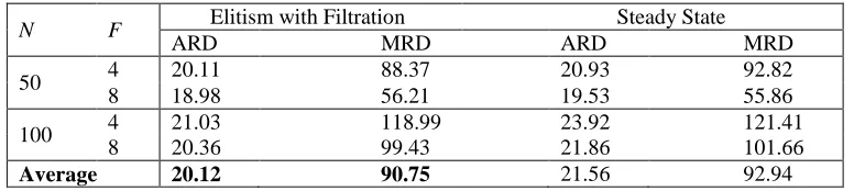
Table 4: Comparison between replacement strategies (15 CPU seconds per run)
The results obtained by the elitism replacement and filtration strategy are better compared to the steady state. In fact, the elitism replacement and filtration strategy can search the solution space in a more efficient manner. The demonstrated computational experiments provide guidelines to design the proposed OCGA. Thus, we apply the optimized crossover and the F-point swap operator to produce offspring in the proposed OCGA. While the elitism replacement and filtration strategy are used to preserve good solutions and to avoid premature convergence.
Competitors
We used four local search algorithms namely SGA, DLTS, RSDM, and MXGA to compare with our proposed OCGA. In the case of SGA a standard 1-point crossover operator is applied to produce two offspring from two selected parents, while a reproduction procedure is used when the crossover does not apply to the selected parents. Also the replacement scheme employed in the SGA is the steady-state replacement scheme.
As for the DLTS, RSDM, and MXGA, all three local search algorithms are proposed by (Lee et al., 2007). The DLTS applies the shift job neighborhood approach and dynamically controls the length of the tabu list during implementation in order to achieve better solution quality. After a move is executed, the job that is shifted is stored in the tabu list, or both jobs are stored if the move is effectively transpose of adjacent
jobs. Thus, a neighbor is tabu if it is generated by shifting one of the jobs in the tabu list. Also an aspiration criterion is used into DLTS, in which if the solution value of a tabu neighbor is better than that for all solutions generated thus far, then its tabu status is overridden.
In the case of RSDM, a steepest descent method using a shift job neighborhood is developed. The RSDM adopts an acceptance rule that allows neutral moves to be made for up to M consecutive iterations where M is a parameter, before terminating the algorithm. Hence, when multiple identical good solutions are found in a single iteration, the RSDM selects a move randomly from the list of the identical good solutions. This strategy is applied to escape the search from falling into the same local optimum.
Finally, the differences between the MXGA and our OCGA are with regards to the use of the crossover operator, swap operator and the mutation operator. The MXGA selects offspring for the population from a candidate list of temporary offspring generated via F-point crossover operator. During the swap operator, a swap point is randomly selected within a parent and the substrings separated by the swap point are exchanged to form a new offspring.
Two mutation operators are used in MXGA: first, an offspring is selected based on an individual mutation probability 𝑝𝑀, then
each element in the selected offspring is N F Elitism with Filtration Steady State
ARD MRD ARD MRD
50 4 20.11 88.37 20.93 92.82 8 18.98 56.21 19.53 55.86
250 visited and altered with a gene mutation
probability, 𝑝𝑚.
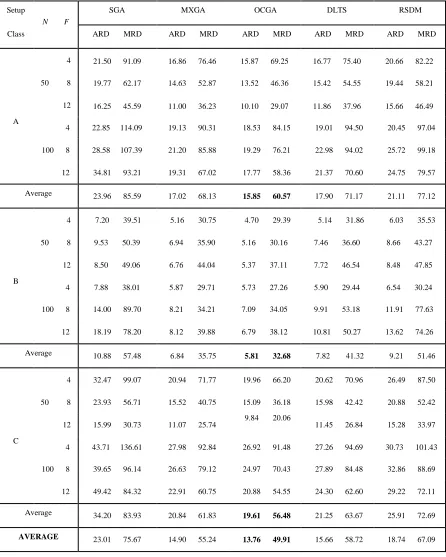
Results and Discussions
In this computational experiment, we used the problem instances described earlier. For each combination of problem instances, 30 runs were performed. In order to have a fair comparison between different algorithms, we employed a duration of 15 CPU seconds per run in this experiment. Table 5 shows the computational results in which for each algorithm, the entries report the average value of ARD and MRD computed over the five problem instances with five combinations of due dates (i.e. 750 runs). For each setup class, the final line gives the average over all values of N and F. The final line of Table 5 gives the overall average value over all setup classes. It is clear from Table 5 that the OCGA performs better than the SGA, DLTS, RSDM, and MXGA algorithms. This indicates that our proposed algorithm is able to produce better quality solutions compared to others. We have also found that computational difficulty as measured by relative deviation from the lower bound increases with problem size. In the case of setup time class C with large setup time, jobs tend to form a large batch size with more jobs in a batch to reduce the need of setup time between batches from different families. Therefore, more jobs will miss their assigned due dates. However, with a small setup time similar to setup time class B, more jobs will meet their respective due dates. Hence when the setup time is small more batches are formed which means fewer jobs are to be processed per batch.To verify the performance of our proposed OCGA compared to other local search methods, a statistical test namely the paired t-test is also applied by using S-PLUS statistical package. First we set up two hypotheses for each two paired samples (i.e. each method and the proposed OCGA are separately two paired samples). The null hypothesis, which assumes the mean of two paired samples are equal and the alternative hypothesis, which assumes the mean of proposed OCGA is less than the mean of
other method for each two paired samples. Note that all assumptions of the test are fully met.
Results show that the lower bounds of 95% confidence intervals for the mean differences between each method and the proposed OCGA are greater than zero, which suggests a positive difference between them. The small p-value (p < 0.001) for the four comparisons, which is highly significant, states that the data are inconsistent with the null hypothesis, that is, the proposed OCGA does not perform equally with other methods. Specifically, with the alternative hypothesis, it can be concluded that the proposed OCGA has a less mean than the other local search methods.
Conclusion
In this paper, we developed an optimized crossover genetic algorithm to effectively solve the problem of 1|𝑠𝑓| 𝐿𝑚𝑎𝑥 . Various
251 Table 5: Comparative computational results (15 CPU seconds per run)
Setup
N F
SGA MXGA OCGA DLTS RSDM
Class ARD MRD ARD MRD ARD MRD ARD MRD ARD MRD
4 21.50 91.09 16.86 76.46 15.87 69.25 16.77 75.40 20.66 82.22
50 8 19.77 62.17 14.63 52.87 13.52 46.36 15.42 54.55 19.44 58.21
12 16.25 45.59 11.00 36.23 10.10 29.07 11.86 37.96 15.66 46.49
A
4 22.85 114.09 19.13 90.31 18.53 84.15 19.01 94.50 20.45 97.04
100 8 28.58 107.39 21.20 85.88 19.29 76.21 22.98 94.02 25.72 99.18
12 34.81 93.21 19.31 67.02 17.77 58.36 21.37 70.60 24.75 79.57
Average 23.96 85.59 17.02 68.13 15.85 60.57 17.90 71.17 21.11 77.12
4 7.20 39.51 5.16 30.75 4.70 29.39 5.14 31.86 6.03 35.53
50 8 9.53 50.39 6.94 35.90 5.16 30.16 7.46 36.60 8.66 43.27
12 8.50 49.06 6.76 44.04 5.37 37.11 7.72 46.54 8.48 47.85
B
4 7.88 38.01 5.87 29.71 5.73 27.26 5.90 29.44 6.54 30.24
100 8 14.00 89.70 8.21 34.21 7.09 34.05 9.91 53.18 11.91 77.63
12 18.19 78.20 8.12 39.88 6.79 38.12 10.81 50.27 13.62 74.26
Average 10.88 57.48 6.84 35.75 5.81 32.68 7.82 41.32 9.21 51.46
4 32.47 99.07 20.94 71.77 19.96 66.20 20.62 70.96 26.49 87.50
50 8 23.93 56.71 15.52 40.75 15.09 36.18 15.98 42.42 20.88 52.42
12 15.99 30.73 11.07 25.74 9.84 20.06 11.45 26.84 15.28 33.97
C
4 43.71 136.61 27.98 92.84 26.92 91.48 27.26 94.69 30.73 101.43
100 8 39.65 96.14 26.63 79.12 24.97 70.43 27.89 84.48 32.86 88.69
12 49.42 84.32 22.91 60.75 20.88 54.55 24.30 62.60 29.22 72.11
Average 34.20 83.93 20.84 61.83 19.61 56.48 21.25 63.67 25.91 72.69
252 References
Aggarwal CC, Orlin JB, Tai RP. (1997) “Optimized crossover for the independent set problem”. Operations Research. Vol. 45, pp. 226-234.
Ahuja RK, Orlin JB, Tiwari A. (2000) “A greedy genetic algorithm for the quadratic assignment problem”. Computers & Operations Research. Vol. 27, pp. 917-934. Allahverdi A, Gupta JND, Aldowaisan T. (1999) “A review of scheduling research involving setup considerations”. Omega, International Journal of Management Science. Vol. 27, pp. 219-239.
Allahverdi A, Ng CT, Cheng TCE, Kovalyov MY. (2008) “A survey of scheduling problems with setup times or costs”. European Journal of Operational Research Vol. 187, pp. 985-1032.
Baker KR. (1999) “Heuristic procedures for scheduling job families with setups and due dates”. Naval Research Logistic. pp. 976-991.
Baker KR, Magazine MJ. (2000) “Minimizing maximum lateness with job families”. European Journal of Operational Research. Vol. 127, pp. 126-139.
Balas E, Niehaus W. (1996) “Finding large cliques in arbitrary graphs by bipartite matching”. In: Johnson DS., Trick MA. (eds.): Clique, coloring and satisfiability: second DIMACS implementation challenge. pp. 29-53.
Balas E, Niehaus W. (1998) “Optimized crossover-based genetic algorithms for the maximum cardinality and maximum weight clique problems”. Journal of Heuristics. Vol. 4, pp. 107-122.
Bruno J, Downey P. (1978) “Complexity of task sequencing with deadlines, set-up times and changeover costs”. SIAM Journal on Computing. Vol. 7, No. 4, pp. 393-404. Graham RL, Lawler EL, Lenstra JK, Rinnooy Kan AHG. (1979) “Optimization and approximation in deterministic machine scheduling diseases: a survey”. Annals of Discrete Mathematics. Vol. 5, pp. 287-326. Hariri AMA, Potts CN. (1997) “Single machine scheduling with batch setup time to minimize maximum lateness”. Annals of Operations Research Vol. 70, pp. 75-92.
Holland JH. (1975) Adaptations in natural and artificial systems. Ann Arbor: The University of Michigan Press.
Jackson JR. (1955) Scheduling a production line to minimize maximum tardiness. University of California, Los Angeles.
Jin F, Song S, Wu C. (2009) “A simulated annealing algorithm for single machine scheduling problems with family setups”. Computers & Operations Research. Vol. 36, pp. 2133-2138.
Lawler EL, Lenstra JK, Rinnooy Kan AHG, Shmoys DB. (1993) “Sequencing and scheduling: algorithms and complexity. In: Graces SC., Rinnooy Kan AHG., Zipkin PH. (eds.): Logistic of production and inventory, Handbooks in operations research and management science”. North-Holland: Amsterdam. Vol. 4, pp. 445-522.
Lee LS, Potts CN, Bennell JA. (2007) “A genetic algorithms for single machine family scheduling problem”. In proceedings of 3𝑟𝑑
IMT-GT 2007 regional conference on mathematics, statistics and applications, 3-5 December 2007, Penang, Malaysia. pp. 488-493.
Mason AJ. (1992) Genetic algorithms and scheduling problems. PhD thesis, University of Cambridge, UK.
Monma CL, Potts CN. (1989) “On the Complexity of scheduling with batch setup time”. Operations Research. Vol. 37, No. 5, pp. 798-804.
Pan JCH, Chen JS, Cheng HL. (2001) “A Heuristic approach for single machine scheduling with due dates and class setups”. Computers & Operations Research. Vol. 28, pp. 1111-1130.
Potts CN, Kovalyov MY. (2000) “Scheduling with batching: a review”. European Journal of Operational Research. Vol. 120, pp. 228-249.
Schultz SR, Hodgson TJ, King RE, Taner MR. (2004) “Minimizing L-max for the single machine scheduling problem with family set-ups”. International Journal of Production Research. Vol. 42, pp. 4315-4330.
set-253 up times”. Computers & Operations
Research. Vol. 35, pp. 2018-2033.
Zdrzałka S. (1991) “Approximation algorithms for single machine sequencing with delivery times and unit batch setup times”. European Journal of Operational Research. Vol. 51, pp. 199-209.