Efficient finite element numerical solution of the variable coefficient fractional subdiffusion equation

(1)

R E S E A R C H

Open Access

Efﬁcient ﬁnite element numerical solution of

the variable coefﬁcient fractional

subdiffusion equation

Lin He

1

_{and Juncheng Lv}

2,3*

*_{Correspondence:}

[email protected];

[email protected] 2_{Henan Geology Mineral College,}

Zhengzhou, China

3_{College of Mathematics and}

Information, Fujian Normal University, Fuzhou, China Full list of author information is available at the end of the article

Abstract

Based on the weighted and shifted Grünwald formula, a fully discrete finite element scheme is derived for the variable coefficient time-fractional subdiffusion equation. Firstly, the unconditional stable and convergent of the fully discrete scheme in

L1(H1)-norm is proved. Secondly, through a new estimate approach, the superclose properties are obtained. The global superconvergence orderO(

τ

2₊_hm+1_{) is deduced}

with the help of interpolation postprocessing technique. Finally, some numerical results are provided to verify the theoretical analysis.

MSC: 65N15; 65N30

Keywords: Subdiﬀusion equation; Weighted and shifted Grünwald formula; Finite element method; Superconvergence estimate

1 Introduction

In the recent few decades, the remarkable applications of fractional calculus in diverse en-gineering fields have been gradually realized and, meanwhile, the discussion of the related fractional partial differential equations (FPDEs) becomes a hot topic of many scholars. For instance, the reader may refer to the work [1–11]. Like traditional partial differen-tial equations, most commonly the exact solutions of the FPDEs are not available. Even if their solutions can be found, they are usually in the form of series, which are difficult to evaluate. So the numerical investigation of the FPDEs has been a vital topic in recent years.

Fractional derivatives are nonlocal operators and they have the character of history de-pendence. When solving approximation solutions for time FPDEs on the current time layer, one needs to retain the information about all the previous time layers, which makes the storage expensive. Based on this aspect, developing high-order numerical methods for solving time FPDEs are quite valuable. In the present studies, we propose high-order methods by first improving the spatial accuracy with the compact difference operator for time FPDEs, which needs few grid points to produce a highly accurate solution. Gao and Sun [12] applied theL1 approximation for the time-fractional derivative and developed a compact finite difference scheme for the fractional sub-diffusion equation. The stability andL∞ convergence are proved by the energy method. Wang and Vong [13,14]

(2)

lished high-order schemes for the fractional diffusion-wave equation and the modified anomalous fractional subdiffusion equation and fractional Klein–Gordon equation, re-spectively.

Another way for developing a high-order method for solving time FPDEs is to improve the temporal accuracy. Recently, a weighted and shifted Grünwald difference (WSGD) op-erator was developed for solving space fractional diffusion equations in [15]. The WSGD operator to approximate the Riemann–Liouville derivative can achieve second-order ac-curacy. Gao et al. [16] presented a new numerical differentiation formula for the Ca-puto fractional derivative, called theL1-2 formula. Then the difference schemes for the time-fractional sub-diffusion equations in bounded and unbounded spatial domains were constructed based on theL1-2 formula. However, they did not give the analysis on the stability and convergence of the obtained schemes. Later, Gao et al. [17] proposed a second-order difference scheme based on the certain superconvergence at some particu-lar points of the fractional derivative by the first-order GL formula. The obtained scheme can achieve the global second-order accuracy in time. Recently, Alikhanov [18] proposed a new difference analog of the Caputo fractional derivative, called the L2-1σ formula.

The stability and convergence of these schemes inL2_{-norm were analyzed by the energy} method.

The finite element method is one of the effective numerical methods for solving clas-sical PDEs. For the FPDEs, finite element method also can be a useful and effective nu-merical method. In recent years, some valuable papers were concerned with the finite ele-ment method for the FPDEs. Roop and Ervin [19–21] investigated the theoretical frame-work for the Galerkin finite element approximation to some kinds of the FPDEs. Jiang and Ma [22] analyzed the finite element method and showed that the optimal convergent rateO(τ2–α₊_N–m_{) can be obtained, where}_m_{measures the regularity of the solution in} space. Jin et al. [23–25] constructed some finite element schemes for solving some kinds of the FPDEs. They proved that those schemes were stable and the numerical solution was convergent. In [26] a fully discrete finite element scheme for solving the two-dimensional space- and time-fractional Bloch–Torrey equations is developed and the stability and con-vergence estimate of the fully discrete scheme are proved. Wang and Yang [27] studied the wellposedness of a variable coefficient conservative fractional elliptic differential equation and its weak formulation. Recently, Ren et al. [28,29] presented two fully discrete schemes for the diffusion equations and diffusion-wave equations, respectively. The unconditional stability and superconvergence error estimates of the obtained schemes are investigated using the integral identities and postprocessing techniques. The optimal time accuracy

O(τ2–α) (0 <α< 1) andO(τ3–α) (1 <α< 2) is obtained, respectively. However, according to current knowledge of the authors, there are few studies on the numerical treatment of FPDEs, high eﬃcient numerical methods of time and space superconvergence analysis are still limited.

(3)

element scheme and establish the corresponding superconvergence error estimate. The method follows the idea of the weighted and shifted GL diﬀerence operators [14, 15]. Based on the equivalence of Riemann–Liouville derivative and Caputo derivative under some regularity assumptions, we derive a second-order accuracy formula to approximate Caputo fractional derivative and the standard Galerkin ﬁnite element method approach for the spatial discretization. The unconditional stability andL1_(H1_{)-norm convergence} are proved rigorously.

The outline of this paper is as follows. In Sect.2, some preliminary numerical formulas and useful lemmas are prepared. In Sect.3, a fully discrete scheme for the variable coeffi-cient fractional subdiffusion equation is developed and the unconditional stability of the obtained scheme is proved. In Sect.4, the superclose and superconvergence analysis for the scheme are presented. In Sect.5, some numerical examples are presented to verify our theoretical results. Some conclusions are given in the last section. Throughout this paper, the notationcdenotes a generic constant, which may differ at different occurrences, but it is always independent of the mesh sizeh, the time step sizeτ. LetWk,p₍_Ω_{) the standard} Sobolev space ofk-differential functions inLp(Ω), its norm by · k,p, and the norm of Hk(Ω) by · k. Whenk= 0, we letL2(Ω) denote the corresponding space defined onΩ with norm · .

2 Preliminaries

In this section, some useful notations, lemmas and formulas will be prepared for the forth-coming work.

For temporal discretization, we divide the interval [0,T] intoN-subintervals withτ = T/N and tk =kτ, k = 0, 1, 2, . . . ,N. Let un=u(x,y,tn). In order to develop a second-order approximation of the Riemann–Liouville fractional derivative, we introduce the shifted Grünwald approximation to the Riemann–Liouville fractional derivative given by (cf. [30])

Aατ,rf(t) = 1 τα

∞

k=0

g_k(α)ft– (k–r)τ, (1)

whereris an integer andg_k(α)= (–1)k₍α

k). Based on the method introduced by [14,15], we suppose thatf ∈C2+α_{(R), then it hold that}

1 +α 2

Aατ,0f(t) –

α 2A

α τ,–1f(t)

=_–_∞RDα_tf(t) +Oτ2 (2)

uniformly holds int∈Rasτ→0. We have

Cn+α(R) =

ff ∈L1(R) and ∞

–∞

1 +|κ|n+αfˆ(κ)dκ<∞

,

(4)

By using a simple calculation the left-hand side of (2) is equivalent to the following

equa-In order to establish fully discrete ﬁnite element scheme, we introduce some notations as follows. We assume thatΩ can be partitioned by a rectangular mesh. Leth={K} be a rectangular mesh overΩ with sizeh. LetVh⊂H01(Ω) be a standard ﬁnite element

whereQm(K) denotes the space of polynomial functions of total degree lower or equal to mwith respect toxandyonK.

Moreover, Ih :C0(Ω¯)→Vh denotes the Lagrange interpolation operator, i.e.,Ih|K ∈ Qm(K) and the interpolation error estimates imply that foru∈Hr+1(Ω) (cf. [31])

u–Ihus≤chr–sur+1, 0≤s≤r, 0 <r≤m+ 1. (4)

3 Stability for fully discrete ﬁnite element scheme

(5)

where 0 < α < 1 and C₀Dα

t denotes the Caputo fractional derivative, the symbol ∇· and∇ denote the divergence and gradient operators, respectively,f(x,y,t) is the given smooth function. It is without loss of generality to assume thatu(x,y, 0) = 0. Ifu(x,y, 0) = φ(x,y)= 0, let v(x,y,t) =u(x,y,t) –φ(x,y) and consider the problem with respect to v(x,y,t). b(x,y) is a smooth and bounded function, which satisﬁes following assump-tion:

0 <β1≤b(x,y)≤β2. (6)

In the current work, we assume that the functionu(x,y,t) can be extended by zero from the time bounded domain [0,T] toR. Noticing the equivalence between the Riemann– Liouville fractional derivative_–_∞RDα

tf(t) with f(t) = 0 whent≤0 and the Caputo frac-tional derivative R

–∞Dαtf(t). Assuming that–∞RDαtu∈C2+α(R) and using (2), we discretize the time-fractional derivative as follows:

R

According to (7), we arrive at the following fully discrete ﬁnite element scheme for the problem (5): ﬁnduk

In order to obtain the stability and convergence of the fully discrete scheme (8), we prove ﬁrstly the following priori estimate.

Theorem 1 Let wk

h∈Vhbe the solution of the following scheme:

⎧

Proof Takingvh=wkhin (9), using Cauchy–Schwarz inequality, we have

(6)

Summing up the above inequality forkfrom 1 ton, we obtain

h= 0, whenτ is suﬃciently small, with the help of Lemma1yields

τ

This completes the proof.

From Theorem1, we can obtain the following stability conclusion.

Theorem 2 The fully discrete ﬁnite element scheme(8)is unconditionally stable with re-spect to the inhomogeneous term f.

4 Superconvergence estimate for the fully discrete ﬁnite element scheme In this section, we discuss the error estimate for the fully discrete scheme. In order to analyze the spatial discretization error, we assume that the solution is suﬃciently smooth. First, let us introduce the following two lemmas.

Lemma 2([32]) Assume that u∈Hm+2₍_Ω_),_{then we have}

_∇(u–Ihu),∇v≤chm+1um+2∇v, ∀v∈Vh. (10)

Lemma 3 Suppose that R

–∞Dαtu∈Hm+1(Ω),Ihu be the ﬁnite element interpolation of u.

29], we similarly obtain the desired result.

By virtue of Lemmas2and3, now we carry out the rigorous error analysis for the fully ﬁnite element scheme (8).

Theorem 3 Suppose that_–_∞RDα

tu∈Hm+1(Ω),ut∈Hm+2(Ω)∩H01(Ω),let ukhand Ihukbe the ﬁnite element solution and ﬁnite element interpolation of u(tk),respectively.Then the following supercloseness estimate holds for1≤n≤N:

(7)

Proof We split the error

Kb(x,y)dx dy, applying the Bramble–Hilbert Lemma (cf. [31]), we have

b(x,y) –A≤chb1,∞. (14)

Using the Cauchy–Schwarz inequality, Lemma2and (14), we arrive at

(8)

Substituting (13) and (15) into (12), applying Lemma3and summing upkfrom 1 ton, we

Noting thatθ0= 0 and applying Lemma1yields the desired result. This completes the

proof.

Furthermore, we can obtain the global superconvergence result of the fully discrete scheme (8) by virtue of a proper postprocessing technique introduced by [32]. For the sake of completeness, we present the construction method of the operatorΠ2h. First we combine four neighboring elements into a big elementK˜ =4_i=1Ki, which has the follow-ing properties (cf. [32,33]): We can deduce the following global superconvergence result.

Theorem 4 Suppose uk_hare the solution of the fully discrete ﬁnite element(8)and under the conditions of Theorem3.Then we have the following result for1≤k≤N:

(9)

Table 1 Numerical errors and convergence orders in temporal direction withh=₂₅₀π atT= 1 for

Table 2 Numerical errors and convergence orders in spatial direction withτ=₁₀₀1 andα= 0.1 at

T= 1 for Example1

π/4 2.7783e-1 1.96 6.4095e-1 0.99 8.8916e-2 2.13 7.3428e-2 1.95

π/8 7.1625e-2 1.99 3.2382e-1 1.00 2.0343e-2 2.04 1.8993e-2 1.96

π/16 1.8037e-2 2.00 1.6239e-1 1.00 4.9636e-3 2.01 4.8653e-3 1.99

π/32 4.5157e-3 2.00 8.1256e-2 1.00 1.2311e-3 2.01 1.2246e-3 2.01

π/64 1.1277e-3 ∗ 4.0636e-2 ∗ 3.0493e-4 ∗ 3.0451e-4 ∗

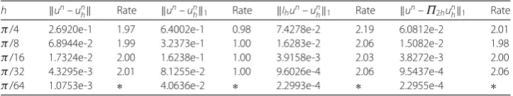
Table 3 Numerical errors and convergence orders in spatial direction withτ=₁₀₀1 andα= 0.3 at

T= 1 for Example1

h un_–_un

h Rate un–u n

h1 Rate Ihun–unh1 Rate un–Π2hunh1 Rate

π/4 2.6920e-1 1.97 6.4002e-1 0.98 7.4278e-2 2.19 6.0812e-2 2.01

π/8 6.8944e-2 1.99 3.2373e-1 1.00 1.6283e-2 2.06 1.5082e-2 1.98

π/16 1.7324e-2 2.00 1.6238e-1 1.00 3.9158e-3 2.03 3.8272e-3 2.00

π/32 4.3295e-3 2.01 8.1255e-2 1.00 9.6026e-4 2.06 9.5437e-4 2.06

π/64 1.0753e-3 ∗ 4.0636e-2 ∗ 2.2993e-4 ∗ 2.2955e-4 ∗

Proof We can deduce from the property (16) and Theorem3that

τ

(10)

Figure 1The exact solution (top) and numerical solution (bottom) for Example1, whenh= 0.05,τ= 0.05,

α= 0.5 andT= 1

Remark 4.1 It should point that using the WSGD operator to approximate R –∞Dαtu(x, y,tk), the temporal derivative provided that ∂

n_u(x,y,t)

∂tn |t=0= 0 (n= 0, 1, . . . , 4), which can be guaranteed in view of the work in [34] and [35], is suﬃcient but not necessary. We will further illustrate this point by numerical experiments (Example2).

Remark4.2 In the present work, we obtain the superclose and superconvergence results inL1(H1)-norm through approach for WSDG fully discrete ﬁnite element scheme, which improve the conclusions in [17,22,29]. It seems that these results have never be seen in the existing literature.

Remark4.3 LetRh:H01(Ω)→Vhbe the Ritz projection operator deﬁned by

b∇(u–Rhu),∇vh

(11)

Table 4 Numerical errors and convergence orders in temporal direction withh=₃₀₀π andβ= 2 at

T= 1 for Example2

α τ un–un_h1 Rate

α= 1/3 1/2 2.8602e-2 2.07

1/4 6.8097e-3 2.03

1/8 1.6620e-3 2.04

1/16 4.0529e-4 2.10

1/32 9.4220e-5 ∗

α= 1/2 1/2 4.4594e-2 2.12

1/4 1.0231e-2 2.06

1/8 2.4506e-3 2.03

1/16 5.9844e-4 2.06

1/32 1.4358e-4 ∗

α= 2/3 1/2 6.1011e-2 2.19

1/4 1.3382e-2 2.12

1/8 3.0810e-3 2.05

1/16 7.4636e-4 2.04

1/32 1.8138e-4 ∗

Table 5 Numerical errors and convergence orders in spatial direction withτ=₁₀₀1 ,β= 2 and

α= 0.1 atT= 1 for Example2

h un–un_h Rate un–un_h1 Rate Ihun–unh1 Rate un–Π2hunh1 Rate

π/4 2.7798e-1 1.96 6.4097e-1 0.99 8.9179e-2 2.13 7.3655e-2 1.95

π/8 7.1673e-2 1.99 3.2382e-1 1.00 2.0417e-2 2.03 1.9064e-2 1.96

π/16 1.8050e-2 2.00 1.6239e-1 1.00 4.9828e-3 2.01 4.8843e-3 1.99

π/32 4.5193e-3 2.00 8.1256e-2 1.00 1.2363e-3 2.01 1.2298e-3 2.01

π/64 1.1288e-3 ∗ 4.0636e-2 ∗ 3.0656e-4 ∗ 3.0615e-4 ∗

Table 6 Numerical errors and convergence orders in spatial direction withτ=₁₀₀1 ,β= 2 and

α= 0.3 atT= 1 for Example2

h un_–_un

h Rate un–uhn1 Rate Ihun–unh1 Rate un–Π2hunh1 Rate

π/4 2.7064e-1 1.96 6.4016e-1 0.98 7.6732e-2 2.18 6.2915e-2 2.00

π/8 6.9390e-2 1.99 3.2374e-1 1.00 1.6960e-2 2.05 1.5732e-2 1.97

π/16 1.7445e-2 2.00 1.6238e-1 1.00 4.0926e-3 2.02 4.0023e-3 2.00

π/32 4.3629e-3 2.01 8.1255e-2 1.00 1.0084e-3 2.04 1.0024e-3 2.03

π/64 1.0865e-3 ∗ 4.0636e-2 ∗ 2.4562e-4 ∗ 2.4523e-4 ∗

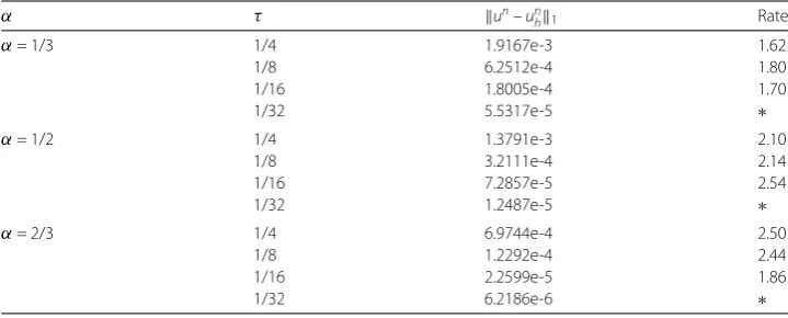
Table 7 Numerical errors and convergence orders in temporal direction withh=₃₀₀π andβ= 3/2 at

T= 1 for Example2

α τ un_–_un

h1 Rate

α= 1/3 1/4 1.9167e-3 1.62

1/8 6.2512e-4 1.80

1/16 1.8005e-4 1.70

1/32 5.5317e-5 ∗

α= 1/2 1/4 1.3791e-3 2.10

1/8 3.2111e-4 2.14

1/16 7.2857e-5 2.54

1/32 1.2487e-5 ∗

α= 2/3 1/4 6.9744e-4 2.50

1/8 1.2292e-4 2.44

1/16 2.2599e-5 1.86

(12)

Table 8 Numerical errors and convergence orders in temporal direction withh=₃₀₀π andβ= 1 at

T= 1 for Example2

α τ un–un_h1 Rate

α= 1/3 1/4 3.1965e-3 1.88

1/8 8.6946e-4 1.79

1/16 2.5118e-4 1.65

1/32 8.0200e-5 ∗

α= 1/2 1/4 7.4822e-3 1.81

1/8 2.1280e-3 1.69

1/16 6.5861e-4 1.60

1/32 2.1679e-4 ∗

α= 2/3 1/4 1.6058e-2 1.74

1/8 4.7995e-3 1.55

1/16 1.6431e-3 1.46

1/32 5.9870e-4 ∗

(13)

Figure 3The error reduction in temporal direction of the scheme (8) for Example3

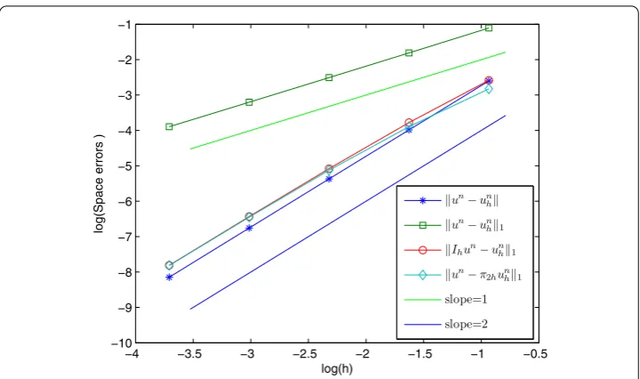
Figure 4The error reduction in spatial direction of the scheme (8) for Example3withα= 0.1

By establishing the relationship between Ritz projection and the linear interpolation as [36], if we chooseRhu instead ofIhu in the supercloseness analysis of Theorem3, the resultτn_k=1Rhuk–ukh1=O(τ2+hm+1) can be obtained.

(14)

Figure 5The error reduction in spatial direction of the scheme (8) for Example3withα= 0.3

5 Numerical experiments

In this section, some test examples based on piecewise bilinear polynomials will be per-formed to illustrate the computational eﬃciency and convergence rate of the proposed schemes.

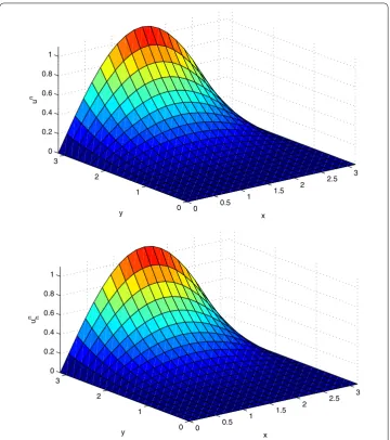
Example1 In (5), setb(x,y) = 1 and letΩ= [0,π]×[0,π] andT= 1. In order to test the convergence rate of the proposed methods, we consider the exact solution of the problem as follows:u(x,y,t) =t2+α_sin_x_sin_{y. Then}_f_(x,_y,_{t) and}_u

0(x,y) are chosen corresponding

to the exact solution, respectively.

Firstly, the numerical accuracies of the fully finite element scheme in time is tested. For differentα, the numerical results are computed using the developed scheme with varying temporal stepsizes and fixed sufficiently small spatial stepsizes. The second-order conver-gence of both the schemes in time can be observed from the data of Table1.

Secondly, the numerical accuracies of the fully finite element scheme in space is verified by the example. With fixed sufficiently small temporal stepsizes, theun_–_un

h,un–unh1,

Ihun–un_h1andun–Π2hun_h1norm errors and spatial convergence orders of the scheme are illustrated in Tables2and3whenα= 0.1, 0.3, respectively. As predicted by the theo-retical estimates, the second-order supercloseness and superconvergence of the scheme in space variable for computing this example are veriﬁed. The ﬁgures of exact solution (top) and numerical solution (bottom) of both schemes are shown in Fig.1.

Example 2 In (5), let b(x,y) = 1 and taking Ω = [0,π]× [0,π], T = 1, f(x,y,t) = [_ΓΓ₍_β(β_+1–+1)_α₎t–α_{+ 1]t}β_sin_x_sin_y_{and initial condition}_u

0(x,y) = 0, then the exact solution of the example is

u(x,y,t) =tβ_sin_x_sin_y,

(15)

α= 0.5 andT= 1

We have pointed out that the condition ∂nu(x,y,t)_∂_tn |t=0 = 0 (n= 0, 1, . . . , 4) is suﬃcient but unnecessary for the numerical accuracy of the proposed schemes. In this exam-ple, we are concerned with the computational results of the fully ﬁnite element scheme for the casesβ = 2, 3/2, 1, respectively. From Table4, we can see that the second-order convergence in temporal direction can be achieved. Tables 5 and 6 show that the supercloseness and superconvergence results in spatial direction can still be achieved.

(16)

unnecessary. The ﬁgures of exact solution (top) and numerical solution (bottom) of both schemes are shown in Fig.2.

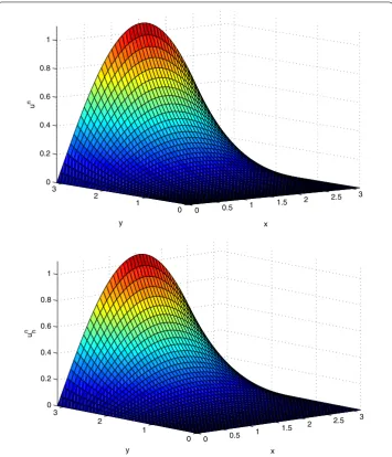
Example3 In (5), takeΩ= [0,π]×[0,π],T= 1,b(x,y) =sinxsiny+ 0.1, the exact solution of the example isu(x,y,t) =t2+α_sin_x_sin_{y. It is not diﬃcult to obtain the corresponding}

forcing termf(x,y,t), and the initial conditionu0(x,y).

We test the numerical scheme (8) for this Example. The results at the timeT= 1 with h=π/300 are reported in Fig.3. We show the temporal errors as the function ofτ for diﬀerent α. The slope is two in good agreement with the theoretical result of Theo-rem 4.2.

The errors obtained by the scheme at timeT= 1 withτ = 1/150 are shown in Figs.4 and 5 with diﬀerent α. It is clear that the second-order supercloseness and super-convergence of the scheme in spatial accuracy are obtained. Similarly, the ﬁgures of exact solution (top) and numerical solution (bottom) of both schemes are shown in Fig.6.

6 Conclusions

In this work, we have developed a high-order approximation fully discrete finite element scheme in time for the variable coefficient time-fractional subdiffusion equation which involves Caputo fractional derivative in time. By using some of the same analytical tech-niques as [28,29], a supercloseness approximation between the interpolation of the ex-act solution and the finite element solution is derived. Then the global superconvergence O(τ2+hm+1_{) in the}_L1_(H1_{)-norm is also obtained with the aid of a suitable postprocessing} method. The global second-order convergence of the obtained schemes in time variable is attainable. In future work, the numerical solutions for the nonlinear fractional differential equations will be investigated.

Acknowledgements

The authors express their sincere thanks to members of the Springer nature waivers team, Springer submission support for their strong help. Also, we would like to thank the anonymous referees for many constructive comments and suggestions which led to an improved presentation of this paper.

Funding

The research is supported by the Foundation of Henan Educational Committee (Grant No. 19A880033).

Competing interests

The authors declare that they have no competing interests.

Authors’ contributions

LH and JCL contributed equally to this work. All authors read and approved the ﬁnal manuscript.

Author details

1_{College of Information Engineering, Zhengzhou Institute of Finance and Economics, Zhengzhou, China.}2_Henan

Geology Mineral College, Zhengzhou, China.3_{College of Mathematics and Information, Fujian Normal University, Fuzhou,} China.

Publisher’s Note

Springer Nature remains neutral with regard to jurisdictional claims in published maps and institutional aﬃliations.

Received: 15 July 2018 Accepted: 1 March 2019 References

1. Podlubny, I.: Fractional Diﬀerential Equations. Academic Press, San Diego (1999)

(17)

3. Shen, T., Xin, J., Huang, J.: Time-space fractional stochastic Ginzburg–Landau equation driven by Gaussian white noise. Stoch. Anal. Appl.36, 103–113 (2018)

4. Zhang, X., Liu, L., Wu, Y.: Multiple positive solutions of a singular fractional diﬀerential equation with negatively perturbed term. Math. Comput. Model.55, 1263–1274 (2012)

5. Li, M., Wang, J.: Exploring delayed Mittag-Leffler type matrix functions to study finite time stability of fractional delay differential equations. Appl. Math. Comput.324, 254–265 (2018)

6. Zhang, X., Liu, L., Wu, Y.: Existence results for multiple positive solutions of nonlinear higher order perturbed fractional diﬀerential equations with derivatives. Appl. Math. Comput.219, 1420–1433 (2012)

7. Zhang, J., Lou, Z., Jia, Y., Shao, W.: Ground state of Kirchhoﬀ type fractional Schrödinger equations with critical growth. J. Math. Anal. Appl.462, 57–83 (2018)

8. Guo, L., Liu, L., Wu, Y.: Existence of positive solutions for singular fractional diﬀerential equations with inﬁnite-point boundary conditions. Nonlinear Anal., Model. Control21, 635–650 (2016)

9. Feng, Q., Meng, F.: Traveling wave solutions for fractional partial diﬀerential equations arising in mathematical physics by an improved fractional Jacobi elliptic equation method. Math. Methods Appl. Sci.40, 3676–3686 (2017) 10. Sun, H.G., Zhang, Y., Baleanu, D., Chen, W., Chen, Y.Q.: A new collection of real world applications of fractional calculus

in science and engineering. Commun. Nonlinear Sci. Numer. Simul.64, 213–231 (2018)

11. Fu, Z.J., Chen, W., Yang, H.T.: Boundary particle method for Laplace transformed time fractional diﬀusion equations. J. Comput. Phys.235, 52–66 (2013)

12. Gao, G.H., Sun, Z.Z.: A compact finite difference scheme for the fractional sub-diffusion equations. J. Comput. Phys.

230, 586–595 (2011)

13. Vong, S.W., Wang, Z.B.: A compact diﬀerence scheme for a two dimensional fractional Klein–Gordon equation with Neumann boundary conditions. J. Comput. Phys.274, 268–282 (2014)

14. Wang, Z.B., Vong, S.W.: Compact difference schemes for the modified anomalous fractional sub-diffusion equation and the fractional diffusion-wave equation. J. Comput. Phys.277, 1–15 (2014)

15. Tian, W.Y., Zhou, H., Deng, W.H.: A class of second order diﬀerence approximations for solving space fractional diﬀusion equations. Math. Compet.84, 1703–1727 (2015)

16. Gao, G.H., Sun, Z.Z., Zhang, H.: A new fractional numerical diﬀerentiation formula to approximate the Caputo fractional derivative and its applications. J. Comput. Phys.259, 33–50 (2014)

17. Gao, G.H., Sun, H.W., Sun, Z.Z.: Stability and convergence of finite difference schemes for a class of time-fractional sub-diffusion equations based on certain superconvergence. J. Comp. Physiol.280, 510–528 (2015)

18. Alikhanov, A.A.: A new diﬀerence scheme for the fractional diﬀusion equation. J. Comput. Phys.280, 424–438 (2015) 19. Roop, J.P.: Computational aspects of FEM approximation of fractional advection dispersion equations on bounded

domains inR2_{. J. Comput. Appl. Math.}₁₉₃_{, 243–268 (2006)}

20. Ervin, V.J., Roop, J.P.: Variational formulation for the stationary fractional advection dispersion equation. Numer. Methods Partial Diﬀer. Equ.22, 558–576 (2006)

21. Ervin, V.J., Heuer, N., Roop, J.P.: Numerical approximation of a time dependent, nonlinear, space-fractional diﬀusion equation. SIAM J. Numer. Anal.45, 572–591 (2007)

22. Jiang, Y., Ma, J.: High-order ﬁnite element methods for time-fractional partial diﬀerential equations. J. Comput. Appl. Math.235, 3285–3290 (2011)

23. Jin, B.T., Lazarov, R., Zhou, Z.: Error estimates for a semidiscrete ﬁnite element method for fractional order parabolic equations. SIAM J. Numer. Anal.51, 445–466 (2013)

24. Jin, B.T., Lazarov, R., Pasciak, J., Zhou, Z.: Error analysis of a ﬁnite element method for the space-fractional parabolic equation. SIAM J. Numer. Anal.52, 2272–2294 (2014)

25. Jin, B.T., Lazarov, R., Liu, Y., Zhou, Z.: The Galerkin ﬁnite element method for a multi-term time-fractional diﬀusion equation. J. Comput. Phys.281, 825–843 (2015)

26. Bu, W.P., Tang, Y.F., Wu, Y.C., Yang, J.Y.: Finite diﬀerence/ﬁnite element method for two-dimensional space and time fractional Bloch–Torrey equations. J. Comput. Phys.293, 264–279 (2015)

27. Wang, H., Yang, D.P.: Wellposedness of variable-coeﬃcient conservative fractional elliptic diﬀerential equations. SIAM J. Numer. Anal.51, 1088–1107 (2013)

28. Ren, J.C., Mao, S.P., Zhang, J.W.: Fast evaluation and high accuracy finite element approximation for the time fractional subdiffusion equation. Numer. Methods Partial Differ. Equ.34, 705–730 (2018)

29. Ren, J.C., Long, X.N., Mao, S.P., Zhang, J.W.: Superconvergence of ﬁnite element approximations for the fractional diﬀusion-wave equation. J. Sci. Comput.72, 917–935 (2017)

30. Meerschaert, M.M., Tadjeran, C.: Finite diﬀerence approximations for fractional advection-dispersion ﬂow equations. J. Comput. Appl. Math.172, 65–77 (2004)

31. Ciarlet, P.G., Lions, J.L.: Handbook of Numerical Analysis, Vol. II: Finite Element Methods (Part 1). North-Holland, Amsterdam (1991)

32. Lin, Q., Yan, N.N.: The Construction and Analysis of High Eﬃcient Elements. Hebei University Press, China (1996) 33. Ren, J.C., Ma, Y.: A superconvergent nonconforming mixed ﬁnite element method for the Navier–Stokes equations.

Numer. Methods Partial Diﬀer. Equ.32, 646–660 (2016)

34. Dimitrov, Y.: Numerical approximations for fractional diﬀerential equations. J. Fract. Calc. Appl.5, 1–45 (2014) 35. Chen, M., Deng, W.H.: High order algorithms for the fractional substantial diﬀusion equation with truncated Lévy

ﬂights. SIAM J. Sci. Comput.37, A890–A917 (2015)