R E S E A R C H
Open Access
Autonomous algorithms for centralized and
distributed interference coordination: a virtual
layer-based approach
Martin Kasparick
1*and Gerhard Wunder
2Abstract
Interference mitigation techniques are essential for improving the performance of interference limited wireless networks. In this paper, we introduce novel interference mitigation schemes for wireless cellular networks with space division multiple access (SDMA). The schemes are based on a virtual layer that captures and simplifies the complicated interference situation in the network and that is used for power control. We show how optimization in this virtual layer generates gradually adapting power control settings that lead to autonomous interference minimization. Thereby, the granularity of control ranges from controlling frequency sub-band power via controlling the power on a per-beam basis, to a granularity of only enforcing average power constraints per beam. In conjunction with suitable short-term scheduling, our algorithms gradually steer the network towards a higher utility. We use extensive system-level simulations to compare three distributed algorithms and evaluate their applicability for different user mobility assumptions. In particular, it turns out that larger gains can be achieved by imposing average power constraints and allowing opportunistic scheduling instantaneously, rather than controlling the power in a strict way. Furthermore, we introduce a centralized algorithm, which directly solves the underlying optimization and shows fast convergence, as a performance benchmark for the distributed solutions. Moreover, we investigate the deviation from global optimality by comparing to a branch-and-bound-based solution.
Keywords: Cellular interference management; SDMA; Distributed algorithms; Autonomous inter-cell coordination; Power control; Network utility maximization
1 Introduction
Increasing bandwidth requirements, not least due to the fast growing popularity of handheld devices with high data rate consumption, bring cellular networks to the brink of their capacity. Until recently, an end to the growth of this demand is not yet in sight. In order to optimally exploit the available bandwidth, current cellular networks experienced a paradigm shift towards frequency reuse-1. Consequently, this leads to an increased susceptibility to interference such that current and future cellular net-works are usually interference limited. This situation is aggravated by a trend towards ever smaller cell sizes. Espe-cially users at the cell-edge are affected by high inter-cell interference (ICI). In theory, fully coordinated networks,
*Correspondence: [email protected]
1Fraunhofer Heinrich Hertz Institute, Einsteinufer 37, Berlin 10587, Germany Full list of author information is available at the end of the article
where neighboring base stations act as a large distributed antenna array, promise a vast boost in performance [1,2]. However, this makes great demands on synchronization and backhaul bandwidth. In fact, the promised gains from such schemes turn out to be hard to implement in prac-tice [3]. As a consequence, distributed schemes for inter-ference mitigation, incorporating joint scheduling and adaptive power allocation, are of utmost interest. How-ever, due to mobile users and varying channel conditions, such algorithms have to be dynamic and able to operate autonomouslya. Moreover, future cellular systems, includ-ing pico and femto cells, must be self-organizinclud-ing to main-tain flexibility and scalability. Therefore, self-optimizing interference coordination schemes are needed.
In this paper, we introduce such schemes with spe-cial focus on cellular space division multiple access (SDMA) networks. All proposed algorithms can be seen as applications of a general radio resource management
framework that configures and optimizes network opera-tion autonomously and that allows us to incorporate ser-vice requirements and performance targets. The frame-work combines the following three essential ingredients:
(i) Network utility maximization (NUM). By
formulating a network utility maximization problem, we steer the system to a desired operating point. This includes fairness goals (like proportional fair and max-min).
(ii) Virtual model. On top of regular scheduling and resource allocation, we maintain a virtual model of the network that captures and simplifies the complicated interference situation in the real world. It comprises a static ‘cooled-down’ version of the network based on long-term gains, thus suppressing the influence of fast-fading. We use this model to obtain granular power control decisions. Thus, it can be seen as a new layer for long-term resource allocation decisions in a cooperative way (including corresponding message exchange).
(iii) Suitable short-term scheduling. Instantaneously, we employ a popular gradient scheduler which is known to asymptotically converge to the solution of the underlying utility maximization problem. The scheduler has to take the power constraints into account (which can be strict or average constraints) that are obtained in the virtual layer to manage interference.
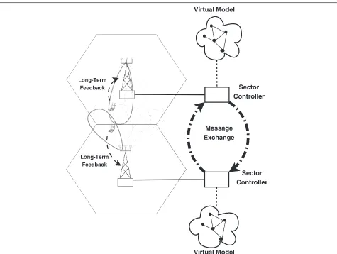
To implement this approach, we equip each base station with an additional sector controller that requires addi-tional (infrequent) long-term feedback from the mobiles. Note, that this is a practical assumption since cur-rently, standardized schemes (such as long-term evolution (LTE)-advanced) also consider advanced feedback con-cepts that are not limited to the serving base station [4]. Moreover, we permit a limited message exchange between the sector controllers. Figure 1 depicts the gen-eral approach. Based upon the long-term feedback, the sector controllers create and update a ‘virtual model’ of the network. The sector controller is thereby just the entity in each base station that takes care of all (virtual) resource allocation and scheduling issues. The main idea of this virtual model is to optimize over ‘virtual resources’, based on long-term averaged versions of true variables, in order to distributively control a rapidly changing complex network. Thus, the virtual model captures the compli-cated interference interdependencies in the ‘real’ network and is used for the control and adaption of power alloca-tions. The virtual model allows each sector to efficiently compute estimates of the gradient of the system utility function with respect to transmit powers of particular resources in the sector, thus allowing local maximiza-tion of the overall utility. More precisely these estimates
are eventually generated by a ‘virtual scheduling’ process. The virtual model and this virtual scheduling process can be considered as an additional virtual layer for resource allocation. The idea is that if user rates improve in the vir-tual layer, they also improve in the real network. Instead of exchanging channel state information (CSI) with all relevant base stations, only the (gradient) information (called sensitivities) that is obtained in the virtual layer needs to be exchanged. The virtual model, being based on average quantities, can be further justified since the goal of the algorithm is to adapt the transmit power lev-els to average interference levlev-els and not to track fast fading.
As mentioned before, we focus on fixed codebook-based schemes in SDMA networks. In particular, we assume that each base station maintains a fixed codebook of a certain size comprising precoding vectors, called ‘beams’. These beams can be used to support multiple users on the same time-frequency resource. Using fixed codebooks is a practical assumption and allows us to compare our algorithms with practical schemes used in current cellular systems.
The optimization within the virtual layer can be orga-nized either in a centralized or in a distributed manner. Clearly, a distributed implementation is favorable but in order to accurately quantify the tradeoffs involved, we also investigate a centralized solution. This does not only provide a valuable benchmark for the distributed algorithms, but may also be a feasible option for small networks, where a central controller is indeed possi-ble. Our centralized baseline algorithm is based on an alternating optimization approach, solving scheduling and power optimization in the virtual control plane sepa-rately. Since user rates are strongly coupled via transmit powers, we employ a successive convex approximation technique to tackle the inherent non-convexity. Due to the non-convex nature of the underlying optimization problem, global optimality cannot be guaranteed. There-fore, we additionally assess the deviation from global optimality by comparing our approach to an optimal solu-tion based on branch-and-bound (BNB) in a simplified setting.
1.1 Related work
Figure 1General network control approach.Each sector controller maintains a virtual model of the network based on long-term feedback. Optimization in this model generates sensitivity messages which are exchanged among sector controllers and which are used to adjust power allocations.
control and scheduling in cellular networks such as [8,9] (see also [10] for an overview). Multicell coordination via joint scheduling, beamforming, and power adaptation is considered in [11]. Thereby, fairness requirements (lead-ing to concave utility functions) are fundamental for current and future cellular standards. The work [12] con-siders joint power allocation and user assignment to cells in the NUM context, taking into account a mixture of concave and non-concave utilities. In [13], a gradient algorithm-based scheme for self-organizing resource allo-cation in LTE systems is proposed. However, a multitude of information has to be exchanged between coordinating sectors.
Although many of the aforementioned references con-sider distributed schemes, none treats resource allocation and interference management in multiuser MIMO sys-tems. By contrast, our framework explicitly aims to exploit the freedom in terms of resource and power allocation offered by SDMA. Thereby, our framework builds upon
and extends the framework introduced in [14,15] for single-antenna (SISO) networks.
[26] considers the derivation of transmit beamformers, also based on interference prices, for dense small cell networks.
1.2 Organization
The paper is organized as follows. In Section 2, we introduce the considered system model, introduce the notation, and describe the optimization problem that we address. In Section 3, we present a virtual control layer for solving this problem and introduce three distributed algo-rithms that are based on different realizations of this vir-tual control plane. In Section 4, we propose an alternative centralized scheme, while in Section 5, we present an opti-mal solution based on branch-and-bound. In Section 6, we present system-level simulation results that evaluate the performance of the distributed algorithms and moreover investigate simpler scenarios to compare these to the cen-tralized and the optimal baselines. Eventually, in Section 7, we state the most important conclusions.
2 System model and notation
We consider the downlink of a cellular OFDMA network, where each cell is sub-divided into three sectors. In total, we haveMsectorsm∈ {1,. . .,M}. Each sector is served by a base station havingnTtransmit antennas with a cor-respondingsector controllerresponsible for user selection and resource allocation. There areI users randomly dis-tributed in the system, each equipped with nR receive antennas. In the following, we assumenR=1. We assume that each user has pending data at all times. LetImbe the
number of users associated to sectorm.
We assume slotted time with time slotst = 1, 2, 3,. . ., called transmission time interval (TTI). In reference to
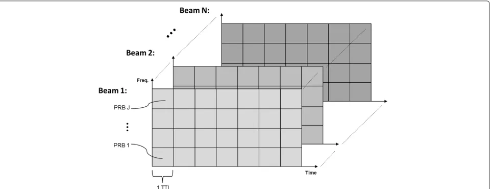
LTE specifications, orthogonal frequency-division mul-tiplexing (OFDM) sub-carriers are grouped into J sub-bands, called physical resource blocks (PRBs)b. For the duration of a time slot, the system is in a fixed fading state from a finite set F. Note, that the assumption of finite fading states is made to foster the analysis. In our simulations, however, we evaluate the performance using established 3GPP channel models (cf. Section 6). Never-theless, the assumption of a finite set of fading states is often used in the literature [27] and can be further justified by the observation that, first, the measurement accuracy of the user devices is limited and, second, there is only a finite number of modulation and coding schemes that the base station can choose from. Fading statel, in turn, induces a finite set of possible scheduling decisionsk ∈ K(l). We denote byπ (l)the probability of fading statel (withlπ (l) = 1). The sector controllers perform lin-ear precoding, where precoding vectors for beamforming are taken (as for example in LTE) from afixed N-element codebookCN := {u1,. . .,uN}which is publicly known.
In the following, we identify a beamforming vector (ub ∈
CnT) by its indexb ∈ {1,. . .,N}. From the sector con-trollers’ perspective, this makes a beam b on a specific PRB ja possible resource for user selection and power allocation. This relationship is depicted schematically in Figure 2. LetPjbmbe the power assigned to beambon PRB jby base station m. This value is determined differently in each of the presented approaches under comparison. In summary, the (non-trivial) task of each sector controller is to find a scheduling decision (being an assignment of available resources on PRBs– to users) and a suit-able power allocation, such that a global network utility function is maximized.
Eventually, we have the following additional notational conventions. Lethmij (t) ∈ CnT be the vector of instanta-neous complex channel gains from base stationmto user ion PRB j(we assume frequency-flat channels within a PRB). Accordingly,hmij (t),u
denotes the scalar product of (beamforming) vectoruand channelhmij (t). The noise power at the mobile terminal is denoted asσ2. Through-out the paper, we label vectors and matrices with bold-faced letters. For the ease of reference, the most important notation used throughout this paper is summarized in Table 1.
2.1 Problem statement
The overall goal is to devise autonomous network control schemes which maximize an overall increasing concave utility function U. The utility function is defined as the sum of sector utility functions Um, which are in turn defined over average user rates X¯m. Consequently, the problem to solve for each sectorm ∈ {1,. . .,M}is given
is a vector
com-prising elements μlijb(k), which represent the rate that useriis assigned on PRBjand beambwhen the system is in fading statel and scheduling decisionk is chosen. They can be zero if the particular resource is not assigned to useri by decisionk. φjklm denotes the fraction of time that scheduling decisionk is chosen on PRBj, provided the system is in fading statel.
In a nutshell, we are not interested in a specific ‘snap-shot’ of the system, but only in ergodic rates. Therefore, a possible control algorithm should not adapt to a specific system state but should be able to optimize the system performanceover time.
Problem (1 to 4) is solved by applying a gradient sched-uler [28] at each time instance. The gradient schedsched-uler chooses the best scheduling decisionk∗according to
k∗(t)∈arg max
Table 1 Important notation
Notation Definition
Pm
jb Power assigned to beambon PRBjin sectorm
¯
Pmjb Average power constraint (‘target’ power) of beambon PRBjin sectorm
¯
Pm(t) Current total allocated power in sectorm
Pmax Maximum total base station power
cjb(k,P¯mj ) Power cost/consumption of beambon PRBj in sectorm
Cm
jb(k) Virtual power cost/consumption of sectorm on beamband PRBj
π(l) Probability of fading statel
K(l) Set of possible scheduling decisions given fading statel
hmij(t) Channel vector from base stationmto useri
on PRBjat timet
¯
hmij Average channel from base stationmto user
ion PRBj
μl
jb(k) Vector of user rates on PRBjand beamb given decisionkand fading statel
¯
Xm Vector of average total rates of users in sectorm
φlm
jk Fraction of time that scheduling decisionkis chosen on PRBjgiven fading statel φm
ijb Fraction of time that useri in sectormis scheduled using beambon PRBj
Gm
ij Long-term gain of userito base stationmfor his best beam on PRBj
Gmijb Long-term gain of userito base stationmfor beambon PRBj
Rm
ij(k) Virtual rate of userion PRBjgiven decisionk
Rj Vector of virtual user rates in PRBj Rmijb Virtual rate of userion PRBjand beamb
Xim Virtual average rate of useriin sectorm
X(t/nv) Vector of virtual average rates attth virtual
jb Sum sensitivity to a power change of beam bon PRBjin sectorm
nj(k) Number of beams that are activated on PRBj if decisionkis chosen
λjb(t) Dual parameter: deviation of power on PRBj and beambfrom the target value
αm
jb(k) Scales target beam powers to instantaneous powers ‘costs’
αm
ijb,βijbm Approximation constants in concave lower bound
The gradient scheduler tracks average user ratesX¯m(t) and updates them after each time slot according to
where the fixed parameterβ > 0 determines the size of the averaging window. The gradient scheduler is known to asymptotically solve the problem (for β → 0) with-out knowing the fading distribution. In case of logarithmic utilities, the gradient scheduler becomes the well-known proportional fair schedulerc.
3 Autonomous distributed power control
algorithms for interference mitigation
We now turn to the distributed power control schemes for autonomous interference management in cellular net-works, which are designed to enable network entities to locally pursue optimization of the global network util-ity. We introduce three basic approaches. It is important to note that all algorithms are special cases of the well-known gradient algorithm [28,29], whose convergence behavior has been thoroughly analyzed. Therefore, we refrain from reproducing this theoretical analysis. How-ever, in Section 6, for illustration purposes, we present numerical results indicating a fast convergence behav-ior. The main difference between the algorithms that we propose is the granularity of power control.
The first algorithm uses an opportunistic scheduler which only adapts the power per frequency sub-band, which is then distributed equally among activated beams. We call this opportunistic algorithm(OA). It leaves full choice to the actual scheduler as to which beam to acti-vate at what time. The scheduler can therefore decide opportunistically (⇒opportunistic algorithm). However, the power budget per PRB which is distributed (equally) among activated beams is determined by an associated control scheme.
The second algorithm is thevirtual sub-band algorithm (VSA), which enforces strict power constraints on each beam by requiring all beams to be switched on all the time (with power values given by the associated control). This has the advantage of making the interference predictable (assuming known power values). However, it leaves only limited freedom for the actual scheduler, whose task is reduced to user selection for each beam. Since a beam is always turned on, it can be treated as an independent resource for scheduling, just like a ‘virtual’ sub-band (⇒ virtual sub-band algorithm).
The third is a hybrid approach, which permits oppor-tunistic scheduling at each time instance but, in addition, enforces average power constraints per beam. We call it cost-based algorithm (CBA). It leaves more freedom for opportunistic scheduling than the virtual sub-band algo-rithm. In contrast to requiring all beams to be used at all times with strict power values, we only require the target beam power values to be kepton average. Thus, instanta-neously, the scheduler is free to make opportunistic deci-sions based on the current system state. In order to assure that the average power constraints are kept, we introduce
an additional cost term into the utility maximization and the gradient scheduler (⇒cost-based algorithm).
We focus on the applicability in different fading environ-ments, comparing the overall performance with respect to a network-wide utility function as well as the perfor-mance of cell-edge users. Thereby, we show that although the algorithms behave differently in different user mobil-ity scenarios, in general, it is more beneficial to impose average rather than strict power constraints.
As we demonstrate later, the three algorithms perform differently with different mobility assumptions on the users. A problem that arises with increased mobility is that the (virtual) model lacks behind the actual network state. Especially when the controllers are restricted to a gradual power adaption process on a per-beam gran-ularity, they might not always be able to fully exploit multiuser diversity. Since the proposed algorithms put different emphasis on opportunistic scheduling in power adaption and resource allocation decisions, they perform differently when facing user mobility and fast fading.
Let us now turn to the control plane, the virtual layer, of the considered algorithms. They all have the follow-ing general procedure in common. The goal of the control plane is to obtain estimates of the partial derivatives of the network utility with respect to the power allocation of particular resources and to adapt the power control policy accordingly. These estimates can be seen as estimates of thesensitivityof the network utility to changes of the allo-cation strategies. Thereby, the alloallo-cation can be, as in the OA of Section 3.1, the power allocation of a PRB which is then divided equally among activated beams. Or it can even be, as in the VSA of Section 3.2, the power alloca-tion of an individual beam. Or it can also be, as in the CBA of Section 3.3, simply an average power constraint of an individual beam, which does not have to be kept at every single time instance.
the sector’s utility. The virtual average rates are based on long-term feedback of averaged channel gains and do not have an immediate physical meaning in the ‘real world’. They are created by a ‘virtual’ scheduler based on ‘virtual’ scheduling decisions. The set of all these rates forms a ‘virtual’ model of the system which is used to derive power adaption decisions.
The question remains how the virtual average rates and accordingly the sensitivities to power changes are cal-culated. Besides the granularity of power control, this virtual model, which can be also seen as a virtual layer for interference mitigation above the actual short-term scheduling, is the main difference between the investi-gated algorithms. In the following, we will discuss this in detail.
3.1 Opportunistic algorithm
OA can be seen as a straightforward extension of the sector gradient (MGR) algorithm in [14] to antenna networks. Although it is designed for multi-antenna networks, it does not perform power control on a per-beam basis (as opposed to the other two algorithms) but gives complete freedom to the sector controllers with respect to the number and choice of beams that are active at every given time instance. The only value that is con-trolled is the power budgetper PRB. Nevertheless, SDMA is applied where multiple users can be scheduled on the same PRB, however on different beams. Consequently, the long-term feedback of users comprises a codebook index (being the maximizing indexb∗in (7)) as well as a corresponding gain troller on PRBj, averaged to eliminate the influence of fast-fading.
The task of finding scheduling decisionknow amounts to determining the best subset of users to be scheduled on a PRB, subject to the constraint that each user can only be scheduled exclusively on its reported beam. Let us define (virtual) user rates (time index omitted), assuming a user is scheduled on PRBj(otherwiseRmij (k)=0), given by is the current power value of PRBjdivided by the num-ber of users scheduled, thus depending on decision k. Moreover,P¯mj G˜mij represents a long-term estimate of the interference of sectormon PRBj(which can be measured by the mobiles).
Having defined the virtual user ratesR, virtualaverage user rates X and sensitivities are derived by virtual scheduling (based on a similar procedure in [14]) as fol-lows. We run the following steps nv times per TTI in
each sector m and for any PRB j. Thereby, the param-eternv determines how long the virtual scheduler runs
before accepting the sensitivities. Consequently, a larger value means more overhead by the virtual layer but better results.
• We determine the virtual scheduling decisionk∗ using a gradient scheduler according to
k∗∈arg max
• We update virtual average user rates according to
X
• We update sensitivities according to
D(jmˆ,m)
Thereby, β1 and β2 are small averaging parameters. Using (8), the derivates in (9) are given by
∂Rmij
Starting with equal power, the adaption of the PRB pow-ers can be summarized as follows. From time to time, the sensitivities are exchanged and summed up by each sec-tor controller for each beam and PRB. Since eachD(jmˆ,m) is an estimation of the sensitivity of sectorm’s utility to a power change in sectormˆ, the summation gives an esti-mate of thenetworkutility’s sensitivity. Then, the power is increased on the PRB with the largest positive sum and decreased on the PRB with the largest negative sum.
3.2 Virtual sub-band algorithm
VSA requires long-term feedback that comprises average link gains per beam and sector from each mobile. We define
CSI, the control plane of VSA responsible for determin-ing the power allocation per beam works as follows. Given average gains in (10), each sector controller calculates corresponding virtual rates according to
Rmijb=:ρ(Fijbm), with
Note that since all beams are activated at all times, we have an additional intra-sector interference term (as opposed to OA), since this interference can no longer be eliminated, e.g., by switching off beams. LetXimbe the vir-tual average rate of useriin sectorm(not to be confused with actual average ratesX¯ in (6)), defined as
Xim=
Here,φ˜mijbrepresentoptimaltime fractions of resource usage for sectorm. They are determined as a solution to the following optimization problem (for fixed virtual user rates):
We rely on an explicit solution to (13) since we can-not apply the virtual scheduling from [14]. This is because the resources for power control (which are now individual beams) are no longer orthogonal but cause interference to each other [30]. Having the virtual user rates, the sec-tor controllers calculate sensitivities to power changes on beams for all sectors (including self ) and beams, given by
D(jbmˆ,m)=
Note that the small coefficient ε > 0 stems from an application of Theorem 1 (which can be found at the
end of Section 3.3) in order to ensure the differentia-bility of problem (13). The such generated sensitivities are exchanged from time to time between all sector con-trollers. Thereby, every sectorkreceivesJ·N sensitivity values from all other(M−1) sectors, in addition to the J·Nvalues from its own sector. Thus, we have
Dmjb=
summing up the sensitivities of all sectors (including itself ) to a power change of beam b on PRB j in sec-tormand which can be either positive or negative. Note that sector indicesmandmˆ in the RHS of (15) are changed compared with (14), since in (14), we are inter-ested in how the beam in sectormˆ interferes with sector m, while in (15), it is of interest how the beam in sectorm interferes with (all) sector(s)mˆ.
SinceDmjb,mˆ represent estimates of the sector utilities to a power change onjbin sector m,Dmjb clearly is an esti-mate of the sensitivity of the system’s utility to a power change on the respective beam. Depending on theDmjb, we can now make a power adjustment which steers the sys-tem operating point towards a greater utility in the virtual model.
By intuition, the algorithm reallocates power to the beams with large positive utility-sensitivity. Note that for numerical reasons, it may be necessary to specify a certain minimum power per beamPminb instead of allowing beam powers to be reduced to zero. In this case, the changes to the algorithmic notation above are straight forward, so we do not explicitly state them here.
3.3 Cost-based algorithm
Since CBA enforces average power constraints per beam, the following additional constraint to the NUM problem (1 to 4) is introduced.
∀b:P¯mjb≥
It includes cost term cjb
k,P¯mj which represents the power cost or power consumption of beamb(on PRBj) given scheduling decision k andP¯mj , which is the total power budget of PRBj. We assume that each beam that is activated gets an equal share of the available total PRB powerP¯mj . Thus, ifnj(k)is the number of beams that are
activated on PRB j if decision k is chosen, the ‘cost’ of activating beambon PRBjbecomes
cjb(k,P¯mj )=
To solve the modified problem (1 to 4 and 16), we also have to modify the gradient scheduler (5 to 6). The modified gradient scheduler now chooses the scheduling decisionk∗according to
k∗∈arg max
Dual parameters λjb(t), measuring the deviation of
powers over time from the target power values on a par-ticular beam, are updated according to the following rule:
λjb(t+1)=
Average user ratesX¯m(t)are maintained and updated as in (6). The above algorithm can be seen as an application of the greedy primal dual (GPD) algorithm presented in [29].
The virtual control plane differs from VSA in the follow-ing. In contrast to the VSA, where every beam is switched on all the time, the situation is different here. To enable the calculation of derivatives of the rates with respect to
beam powers (needed in (22)), we introduce scaling fac-torsαm
jb(k), which scale target beam powersP¯mjbto powers
‘costs’eCm
jb(k)that are instantaneously used by the virtual
scheduler. Thus,αmjb(k)P¯mjb=Cjbm(k).
Given average gains (10) as in VSA, the sector con-trollers calculate (virtual) user rates given by
Rmijb(k)=ρ
Virtual average user rates are calculated by CBA as follows:
Again,φ˜jkmare optimal time fractions of resource usage for sector m; however, in contrast to VSA where those time fractions were calculated explicitly, CBA uses the approach of OA to determine the virtual average rates (and implicitly the time fractions) throughvirtual schedul-ing. As before, to distinguish real and virtual scheduler, we use capital letters for virtual scheduler quantities when-ever possible. In each TTI, the virtual scheduler performs nv scheduling runs. In each run, the following steps are
carried out on each PRBj:
• We determine thevirtual scheduling decisionk∗ similar to (17).
• We updatevirtual average rates similar to (6). • We update thevirtual average power costs for each
beambsimilar to (18).
• We update sensitivities for each beamband sectormˆ (β2>0small) according to
Using (19) to (20), the derivatives in (22) are given by
The power adaption is then carried out similar to the other algorithms. For each resource, each sector sums up
values D(jbmˆ,m) from all sectors and increases the power level on the beam with largest positive sum while decreas-ing the power level on the beam with largest negative sum. However, CBA adapts only power constraints per beam, not actually used beam powers.
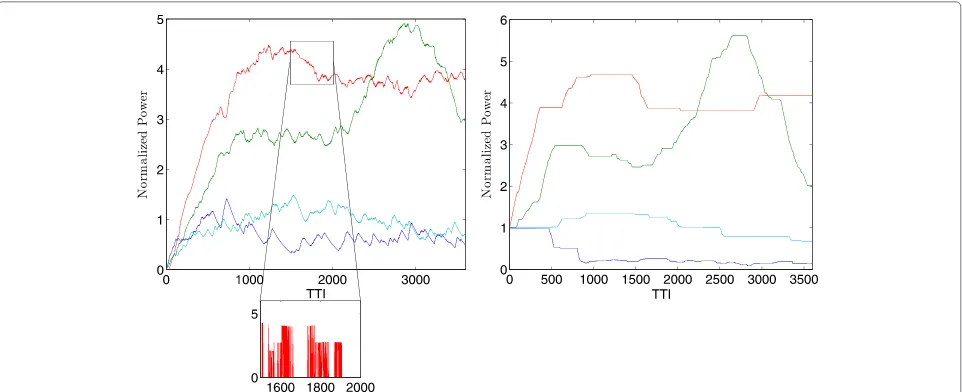
Figure 3 gives a sketch of power trajectories using the simulation environment described below, in Section 6.1. To find out whether CBA really holds the average power constraints, we exponentially average instantaneously used powers per beam with the same time constant used for scheduling and compare the result to the target power values determined by the virtual model. The left side of Figure 3 shows the averaged powers, as actually used by the ‘real’ scheduler, while the right side shows the tar-get power values determined by the virtual scheduling procedure. Note that since scheduling is opportunistic, instantaneously, the power levels fluctuate highly and beam powers can differ from the target values (or a beam can be completely turned off ). This is illustrated by the ‘zoomed-in image’ in Figure 3 (left), where actual powers without averaging are shown. It turns out thaton average, the power constraints are kept remarkably well.
Apart from the intuitive benefits of instantaneously allowing opportunistic scheduling, we observe that from a practical point of view, average power constraints are further justified since hybrid automatic repeat request (HARQ) coding is essentially performed over multiple successive transmissions.
In all three presented algorithms, naturally, questions arise regarding differentiability. Note that the problem to be solved by each sector controller is given in (13). Due to the maximum operator, it might not be differentiable everywhere even with the utility function being differen-tiable. Therefore, let us define a slightly modified version of problem (13), given by
fε(R):=max φm
ijb
i
Um ⎛
⎝
j
b
φm ijb
1−ε
Rmijb ⎞ ⎠. (23)
One can show the following:
Theorem 1. Let0< ε <1be finite and Umbe an
increas-ing concave utility function, defined in (0,∞). Then, the family of functions fε(R)(defined by (23)) with Rijb≥c>0
(∀i,j,b) is differentiable everywhere and converges for any sequenceεn → 0to f in (13) (which is continuous) in the
uniform sense.
Proof. The proof can be found in Appendix 1 .
By Theorem 1, we can replace our utility function with a smooth, uniformly convergent approximation, which can be locally maximized in the power control loop. Note that this replacement is already incorporated in the calculation of sensitivities (Equation 14).
4 An alternating optimization-based approach
Given the distributed nature of the above presented algo-rithms, the question arises: Can a centralized controller do
better? Therefore, in the following, we want to compare the algorithms of Section 3 with a centralized solution.
The optimization problem which the virtual controller has to solve is given by
max As described in Section 3, the power allocation problem is so far solved using a distributed gradient ascent proce-dure. However, when we allow a centralized controller for the network, we can instead solve (24 to 26) directly each time a power update is desired and use the resulting power allocation directly for actual resource allocation.
Obviously, problem (24 to 26) is highly non-convex. In the following, we try to solve the problem by alternat-ing the optimization in P (holding constant) and (holdingPconstant). We therefore have a scheduling sub-problem and a power allocation (PA) sub-sub-problem. The overall procedure is summarized in Algorithm 1.
Algorithm 1 Alternating optimization-based virtual layer
1: initialize counterτ =0, select feasible(0)andP(0) arbitrarily
2: repeat
3: τ ←τ+1
4: solve scheduling sub-problem using fixedP(τ−1) and obtain(τ)
5: solve SCA-based power allocation sub-problem using fixed(τ)and obtainP(τ)(Algorithm 2)
6: untilconverged
7: useP(τ)to update power allocation in network
Since the scheduling sub-problem is convex (cf. Lemma 2), we only have to care about the power allo-cation sub-problem. We try to tackle this problem by a successive convex approximation(SCA) approach similar to [17]. The sub-problem inPis still highly non-convex. However, using Lemma 3, we obtain a convexified version of the power allocation sub-problem.
Lemma 2. With constantP, optimization problem (24-26)
is a convex optimization problem in.
Proof.The proof follows since non-negative weighted addition and scalar composition preserve concavity [31].
Lemma 3. Using a concave lower bound (assuming
appro-priately chosen constants) to the user rates, given by ˜
Rmijb:=αmijblog(Fijbm)+βijbm ≤Rmijb, (27)
(with equality holding when approximation constants are
chosen as αijbm = F
ijblog(Fijbm)) and a logarithmic change of variables given
byP˜mjb=log(Pmjb), the modified PA sub-problem
is a convex optimization problem.
Proof.The proof can be found in Appendix 2 .
The SCA procedure is summarized in Algorithm 2.
Algorithm 2 SCA-based power allocation sub-problem 1: initialize counterτ =0,α(0)=1; β(0)=0
The algorithm converges when the tighten step (30) does not produce any (significant) changes. Being based on an inner approximation framework by Marks and Wright [33], it can be shown that Algorithm 2 converges at least to a KKT point of the PA sub-problem.
5 Approaching global optimality: comparison
with branch-and-bound
It is known that the underlying optimization problem is non-convex; thus, the gradient ascent-based algo-rithms presented in Section 3 as well as the alternating optimization-based algorithm of Section 4 will most likely converge to a local maximum. Thus, although simulation results (cf. Section 6) show already high gains in utility, the question remains how good the solution found actually is, that is how much of the achievable performance gains is actually realized?
To simplify the analysis in this section, we restrict our-selves to the single-antenna case (which reduces all algo-rithms to MGR in [14]). The main difficulty of the analysis is that even in this simple setting, the underlying problem
f(P,)=max
convex (even in the two-sector, two-user case). Moreover, since this is essentially a joint optimization in time frac-tionsand power valuesP, the complexity is significantly higher than with power control only. To gain insight into the deviation from the optimal solution of (31 to 33), we compare our algorithm’s performance in the simpli-fied setting with a (near) optimal solution based on BNB. Although computationally very expensive, it gives us a good impression on how much of the achievable perfor-mance is actually reached. We assume, without loss of generality, that the maximum sum power available in each cell in (33) is normalized to one.
Branch-and-bound is a standard algorithm for global optimization, which creates a search tree where at each node, an upper and a lower bound to the problem are evaluated. Details can be found for example in [34]. It is based on constantly sub-dividing the feasible parameter region and for each node of the resulting tree calculating the upper and lower bounds to the objective function. For ease of notation, we will combine all parameters to our objective function in one vectorPˆ =(p1,. . .,pn). LetP(0)
denote our initial parameter region. This region forms a
convexn-dimensional polytope withVextreme points (or vertices)Pˆv. We collect the corner points of polytopeP(0)
in set V(0). Consequently, the parameter region associ-ated with nodelis denoted asP(l)with associated vertices V(l).
Due to the structure of the constraints, we have n2 parameter pairs with independent constraints. Each of the parameter/constraint pairs form a (two-dimensional) sim-plex. When branching, we split the parameter region of node l, P(l), in sub-regions P(l+1) and P(l+2) by
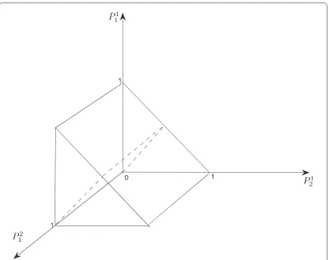
split-ting the longest edge among the edges of all (n2) simplexes together. Doing so, we divide the parameter region into two sub-regions of equal size. Figure 4 visualizes the above-stated procedure by showing the simplex created by two interdependent power values together with an inde-pendent third dimension. The dashed line indicates the splitting into two sub-polytopes.
Below, we explain how the upper and lower bounds to the sub-problems are found. It is well known that the Shannon rate can be written as a differ-ence of concave functions fijm(P) − gijm(P), with fijm
. Using this, our non-concave objective function (31) can be rewritten as
ˆ
is not concave). However, we can define the concave
func-Equation 35 is still not concave since it includes a sum of a concave function (f˜ijm(Pˆ)) and a convex function
Using this definition, the (convex) optimization problem we have to solve in order to obtain our upper bound (at nodel) is given by
the number of vertices collected inV(l).We use three
dif-ferent approaches to obtain a lower bound at nodel. The first lower bound is obtained by taking the maximum of the objective function values at each of the corner points of the respective parameter region. Second, we evaluate the optimal parameter vector from calculating the upper bound. Third, we use a standard solver to compute a (local) optimum of the original non-convex problem. If one of the three methods leads to a higher value, the current global lower bound is replaced.
6 Numerical evaluation
In this section, we present numerical results to evaluate the distributed algorithms of Section 3 as well as the cen-tralized and BNB-based solutions of Section 4 and Section 5, respectively.
6.1 System-level simulations
In order to compare the performance of the three algo-rithms in a setting close to practice, we conduct system-level simulations based on LTE.
6.1.1 Simulation setup
The general simulation setup can be found in Table 2. We employ a grid of seven hexagonal cells, each comprising three sectors (to ensure equal interference conditions for each sector, a wrap-around model is used at the system borders). Users are distributed randomly over the whole area; thus although we have, say, 210 user in total, lead-ing to an average of ten users per sector, some sectors have a higher load than others. A detailed description of the precoding codebook can be found in [35]. As chan-nel model, we use the WINNER model [36], Scenario C2. All simulations are performed with realistic link adapta-tion based on mutual informaadapta-tion effective SINR mapping (MIESM); moreover, we use explicit modeling of HARQ (hybrid automatic repeat request) using chase combining. For efficiency reasons, we simulate a limited number of PRBs (J = 8) compared to a real-world system; however, the results are expected to scale to a higher number of PRBs.
6.1.2 Baseline algorithm
As baseline, we use a non-coordinative scheduling algo-rithm called greedy beam distance (GBD) algoalgo-rithm, with a codebook size of 3 bits (eight beams). GBD requires feedback from each user, comprising a CDI and a chan-nel quality information (CQI) value. Note that the CQI is only an estimate of the users’ SINR values in case the user alone is scheduled on the PRB (with full power), since the scheduling decisions cannot be known in advance. Thus, it does not contain intra-sector interference. Moreover, it contains only an estimate of the inter-sector interfer-ence. On each PRB, the users are greedily scheduled on their best beams (using their proportionally fair weighted CQI feedback as utility). Thereby, a minimum beam dis-tance has to be kept, in order to minimize the interference between users scheduled on the same PRB. This distance
Table 2 General simulation setup
Parameter Value
Number of sectors (M) 21
Total number of terminals (I) 105 to 315
Mobile terminal velocity 0 km/h, 3 km/h
Number of PRBs (J) 8
Number of beams (B) (coordination) 4
Number of beams (B) (baseline) 8
Base station antennas(nT) 4
Number of terminal antennas (nR) 1
Simulation duration 10,000 TTI
Power adaption step size () 0.5% of the initial power
Traffic model Full buffer
is based on a geometrical interpretation of beamforming. It means that given a user is scheduled on a certain beam, adjacent beams (up to a certain ‘distance’) are blocked and users that reported one of those beams are excluded from the list of scheduling candidates for the respec-tive PRB. We use a minimum distance of 3, that is, with the used eight-beam codebook at most three users can be scheduled on the same PRB. Of course, no adaptive power allocation is performed; the power is distributed equally among the PRBs (and further among the thereon scheduled users).
6.1.3 Simulation results
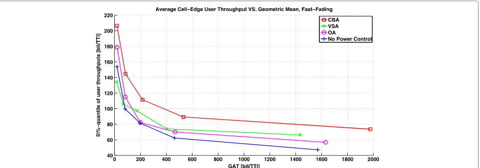
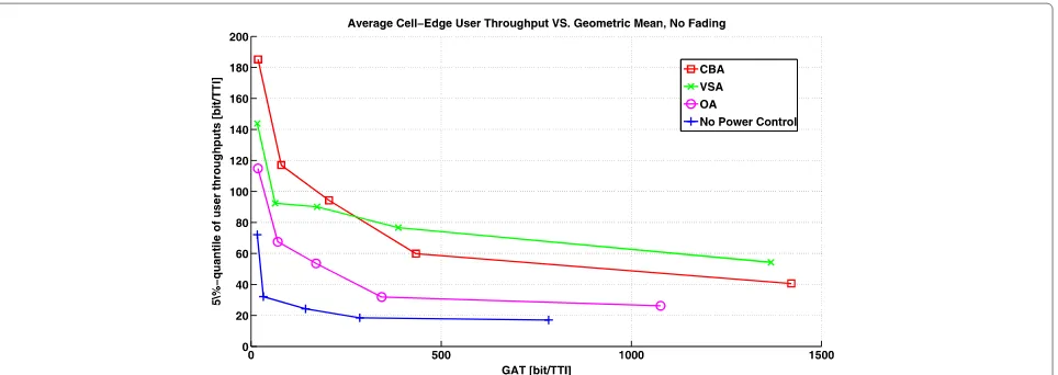
We use two essential performance metrics for our com-parison. First, since we have a system-wide proportional fair utility, we compare the geometric mean of average user rates (GAT) as a measure of the increase of theoverall utility. The equivalence of maximizing GAT and sum util-ity can be seen when observing that the geometric mean of some set of values is equal to the exponential average of the logarithm of the values. Therefore, the sum of log-arithms is maximized precisely if the geometric mean is maximized. Second, the performance of cell-edge users, which we measure by the 5% quantile of average user throughputs, is a natural benchmark for each distributed base station coordination algorithm.
Figure 5 shows cell-edge user throughput over GAT for the evaluated algorithms with user mobility (and there-fore with fast fading), while Figure 6 depicts the simulation results in a setting without user mobility. We compare the three approaches of Section 3 to the uncoordinated baseline of Section 6.1.2. Thereby, for each algorithm, the performance is evaluated for different average number of
users per sector. More precisely, from left to right, the markers in the figure represent an average number of 5, 8, 10, 12, and 15 users per sector (corresponding to total numbers of 105, 168, 210, 252, and 315 users in the net-work, respectively). Obviously, increasing values on the ordinate corresponds to increased fairness (with respect to our 5% quantile metric), while higher values on the abscissa correspond to a higher sum utility (with respect to our GAT metric). In both figures, we observe that a higher number of users lead to increased sum utility (an effect called multiuser diversity) while the cell-edge users (represented by the 5% of users with lowest throughput) suffer from a reduced performance (due to an increased competition for resources).
In case of user mobility (Figure 5), we observe that CBA clearly outperforms the other algorithms. In fact, for every simulated user density, either the 5% fairness (low user densities) or both metrics are improved (higher user densities). For example, in the case of 210 users in the net-work (corresponding to the third marker on the curves in Figure 5), the CBA algorithm improves the performance with respect to GAT by about 10% and in cell-edge user throughput by more than 35%. It can also be observed that the VSA algorithm works best at high user densities, while in case of only a few users in the cell, the OA algo-rithm (which requires the least overhead with respect to additional feedback and signaling) and even the no-power control baseline show a better performance, at least with respect to the cell-edge performance. The decreased GAT shown by VSA in the fading case is basically the cost of leaving no freedom to the schedulers for opportunistic scheduling, but to strictly specify the powers to be used for all beams and time instances.
Figure 6Cell-edge user throughput vs. GAT in a static environment.The averaged cell-edge users’ throughputs vs. the geometric mean of users’ throughputs are plotted for a scenario without user mobility. Thereby, the proposed three distributed algorithms are compared with a baseline algorithm without coordination. For each algorithm, the total number of users in the network is varied. In particular, the markers in the figure, from left to right, represent an average number of 5, 8, 10, 12, and 15 users per sector. This corresponds to total number of 105, 168, 210, 252, and 315 users in the network, respectively.
Figure 6 depicts the simulation results in a setting with-out user mobility. We can see that OA offers already quite high performance gains, both in GAT and in cell-edge user throughput, although being the least complex algorithm. However, the performance is even further improved by the other two algorithms. VSA can improve especially the gains of cell-edge users, for example, in the case of 210 users in the network to more than 200% compared with no-power control. However, CBA again shows the best performance, significantly improving the global utility compared with VSA (and even more compared with no-power control). Again, this gain increases with increasing number of users in the network.
Besides the performance, the speed of convergence is of large practical interest. To illustrate this, Figure 7 shows the GAT metric for all algorithms over time for
the case of stationary users (with 210 users in total). It can be seen that the fastest convergence is achieved by the OA and VSA algorithms, while the CBA algorithm, which in the end achieves the highest GAT, needs about 3,000 TTIs to converge. This is expectable, since the scheduler has to follow the power values obtained from the virtual layer only on average; thus, it always ‘lacks behind’ the adaptation of the virtual model. Regardless of which algorithm performs best, it is of general impor-tance that distributed power control algorithms do not only work in a specific environment but can adapt to changing network conditions (which, of course, is also related to the notion of convergence). Figure 8 demon-strates this autonomous adaptation ability by showing the cell-edge user throughput over time (exemplary for CBA in the static case) for multiple consecutive drops,
Figure 8Cell-edge user throughput over time for consecutive drops, no user mobility.The green line represents the CBA algorithm, while the red line indicates the baseline without power control. Multiple consecutive drops with a duration of 2,500 TTIs are shown.
where, in each drop, a new user location and assign-ment pattern are generated. It can be observed that the the performance is improving very fast compared to the baseline.
6.2 Performance of centralized solution based on alternating optimization
Subsequently, we investigate the performance of the cen-tralized scheme based on alternating optimization (AO), as introduced in Section 4. For this, we compare the performance with that of the distributed solution. More precisely, we use the VSA algorithm of Section 3.2. Note that the only difference between the subsequently inves-tigated algorithms is the power adaptation procedure. While in the distributed solution (in subsequent figures denoted as VSA), the power is adapted gradually based on the exchange of sensitivities, in the centralized solu-tion (in subsequent figures denoted as AO), the solu-tion to the optimizasolu-tion problem in the virtual layer
is directly used to globally update the power alloca-tion. We are predominantly interested in the convergence speed of the geometric mean of average user rates in the different approaches and the relative performances in different signal-to-noise ratio (SNR) regimes. More-over, we investigate both a static setting without mobil-ity and a setting where a user moves at a velocmobil-ity of 3 km/h.
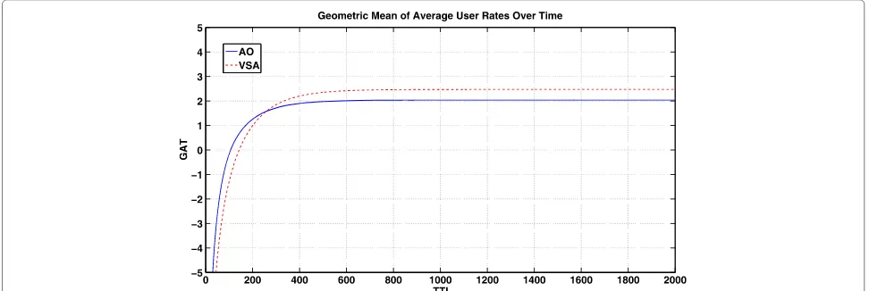
In Figure 9, we compare the behavior of the AO and the distributed approach for constant channels. In gen-eral, it can be observed that the convergence speed of the average rates using AO is slightly faster. Often, both algo-rithms converge to the same solution; however, this is not necessarily always the case (as shown in Figure 9).
Figure 10 compares the performance of AO-based and gradient ascent-based solution in a setting with moder-ate user mobility. It can be observed that the convergence speed of the centralized scheme is still slightly higher than in the distributed case, and in most cases, the centralized solution outperforms the gradient-based approach (how-ever, at a much higher complexity). An interesting effect that can be observed is that the influence of the initial state on the outcome of the distributed solution is significant. This is also depicted in Figure 10. Note that the only differ-ence between the solid and the dashed red line in Figure 10 lies in the initial power values. In the first case, we start at a minimal power assigned to all sub-carriers (note that for technical reasons, it is not possible to assign exactly zero power to the resources) and in the latter case, we start at an allocation where power is distributed evenly among the resources.
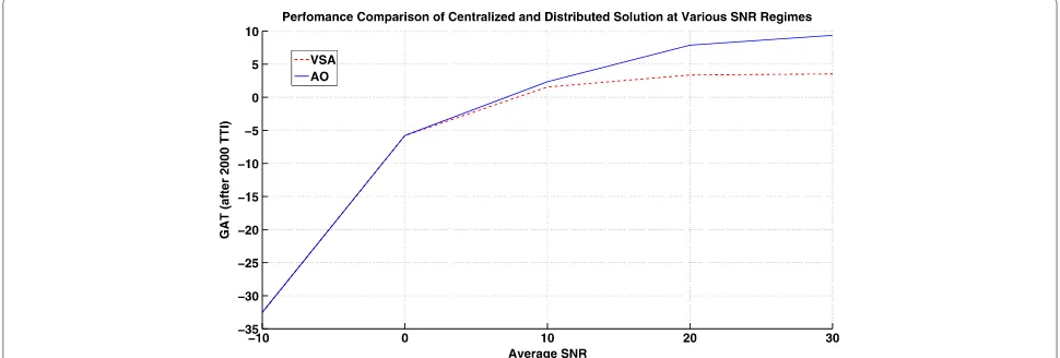
In Figure 11, it can be observed that the gains from the centralized solution are higher in high-SNR regimes. While at low SNRs, when the system is essentially noise-limited, both approaches converge to the same solution; in high-SNR regimes, when the system is essentially
Figure 10Comparison of centralized and distributed virtual control at moderate mobility.The geometric mean of the average user rates is shown in a fast-fading scenario. The centralized baseline (blue) is compared to the VSA algorithm (red) with different initial power allocations.
interference-limited, the direct AO-based optimization outperforms the gradual power adaptation.
In summary, the centralized solution has some clear advantages. First, it is invariant to the initialization of the system and is thus able to adapt very fast to changing environmental conditions. Second, especially when the channels are varying fast and the SNR is high, the central-ized scheme offers a higher performance in comparison to the distributed scheme. However, one should note that at realistic SNRs, the distributed solution still achieves almost the same performance and at the same time scales smoothly with the network size, while a central-ized solution can only be implemented in very restricted scenarios.
6.3 Global optimality
In the following, we compare the performance of the distributed algorithm to an (nearly) optimal solution
based on BNB. To simplify the analysis in this section and due to the high complexity of the BNB algorithm, we restrict ourselves to the simple case of two sectors with two users (no mobility) and two PRBs and a single antenna.
Given a certain toleranceε, BNB converges to an opti-mal solution of (31). However, it has exponential complex-ity and is therefore only feasible in very small settings. We compare our distributed coordination algorithm with an equal power non-cooperative scheduler and the BNB algorithm described in Section 5.
In Figures 12 and 13, the blue line represents the GAT obtained with the coordination algorithm, while the red line represents the outcome of a non-cooperative equal-power scheduler. The solid black line indicates the out-come of BNB. Finally, the dotted black line depicts the configuredεtolerance. Thus, the true optimum is guar-anteed to lie in between the solid and dotted black lines. To get an overview of the performance in different sce-narios, we investigate three different settings, namely, a setting with weak interference, a setting with approxi-mately equal interference, and a setting with high inter-ference. In Figure 12, the left marker corresponds to the weak interference case, the middle marker to the case of equal interference, while the right marker corresponds to the case of strong interference. The weak interference is characterized byGmij > Gmij(m = m) for alli,j,m,m; thus, for all users, the link gains to the serving base sta-tion are higher than the gains to the interfering base station. Note that this is, from a practical point of view, the more interesting case since due to handover algo-rithms, most of the time, the gains to the own base station are stronger than to the interferers. It can be observed that the distributed power control performs quite well since we see a significant improvement over equal power scheduling. Moreover, the distributed power control
Figure 12Comparison of the distributed power control with BNB solution for different interference regimes.
appears to realize already a large portion of the available gains.
In the ‘equal’ interference case, the gains to the inter-fering base stations are roughly the same as the gains to the own base stations; thus, Gijm ≈ Gmij(m = m) for alli,j,m,m. It can be observed that the power control algorithm leaves a larger portion of the available performance gains unused, compared to the weak inter-ference case, although it shows significant improvements over non-cooperative scheduling.
The strong interference case is characterized byGmij < Gmij(m =m), for alli,j,m,m; thus, for all users, the link gains to the interfering base stations are higher than the gains to the ‘own’ base stations. Here, the gap in the non-cooperative algorithm’s performance, compared to the BNB result, is significantly worse than in the other cases. By contrast, the power control algorithm shows roughly the same performance gap than in the case of equal gains. Again, to illustrate the convergence, Figure 13 gives an example of the performance over time (here, for the weak
Figure 13Comparison of distributed power control with the BNB solution.Weak interference example.
interference case). Obviously, the power control algorithm converges to a local maximum soon.
7 Conclusions
We proposed and compared three distributed algorithms for autonomous interference coordination in cellular SDMA networks. The algorithms are based on a virtual layer that models the interference interdependencies in the network and gradually adapts power control levels. The proposed algorithms differ in granularity of power control, required feedback, signaling overhead, and the virtual model itself. System-level simulations indicate high gains both in overall utility and in cell-edge user through-put for all three algorithms in static environments without user mobility. While VSA offers a very fine granularity of power control on a per-beam level, it suffers from the lack of freedom to instantaneously perform power allocation in an opportunistic manner. In fact, in an envi-ronment with significant user mobility, only CBA achieves significant gains in both metrics. This demonstrates the superiority of CBA’s approach to enforce average power constraints but instantaneously allowing opportunistic scheduling. Comparisons to a centralized benchmark scheme reveal that although the convergence of the cen-tralized scheme is much faster than in the distributed case, the performance in overall utility is comparable.
Endnotes
aNote, that in this paper, we use the term autonomous
not in the sense of an autonomous operation of the different network entities, such as base stations, but to the ability of the network to find a suitable operating point without the needed of prior planning or human interaction.
bEach PRB consists of a fixed number of OFDM
symbols in time and has a total length of 1 TTI. cWe use
ilog(X¯im)as sector utility in this paper,
leading to a proportional fair operating point. dTo reduce messaging overhead, sector controllers
could limit the message exchange to strongest interferers, e.g., consider only neighboring base stations.
eTo avoid confusion, we denote variables belonging to
the real scheduler with lower case symbols, and variables from the virtual scheduler with corresponding upper case symbols.
Appendices
Appendix 1: proof of Theorem 1
First, we show that fε(R) is everywhere differentiable. For this purpose, we use the following Lemma 4 and set H(x,y):=U(R,).
Lemma 4. Consider a function H(x,y), x∈ [a1,a2], y ∈
that H(x,y)and its partial derivative on x are continuous, and H(x,y)is concave in x (for each y) and strictly concave in y (for each x). Then, the function
ϕ (x)=max
y H(x,y) (36)
is continuously differentiable in [a1,a2]. (This can be
generalized to the multi-dimensional case. Namely, the domains[a1,a2]and[a3,a4]can be replaced by arbitrary
convex compact sets in finite-dimensional vector spaces, and derivatives replaced by gradients).
Note, that Lemma 4 cannot be applied directly to (13) since strict concavity inyin this case is not given. Clearly, R and are compact since φijb ∈[ 0, 1] and Rijb ∈ [c,B] ,B < ∞,c > 0. Moreover, the concavity of U follows by definition. Now, we have to show thatfε(R) con-verges for any zero sequenceεn→0 tof. First, fix a zero
sequenceεn∗. Moreover, we define a sequence of functions
fn(R):=max
of continuous functions and K being a compact metric space) converges pointwise tof (f : K →Rbeing a
con-Appendix 2: proof of Lemma 3
Following the approach in [17], the convexity of optimiza-tion problem (28 to 29) can be easily shown by noting that
˜
where log(F˜ijbm)can be further decomposed into
log(Gmijb)+ ˜Pmjb−log
Due to the convexity of log-sum-exp [31], the term
log
is convex, and thus, R˜mijb is concave. Noting that non-negative weighted addition and scalar composition pre-serve concavity concludes the proof.
Competing interests
The authors declare that they have no competing interests.
Author details
1Fraunhofer Heinrich Hertz Institute, Einsteinufer 37, Berlin 10587, Germany. 2Technische Universität Berlin, Einsteinufer 25, Berlin 10587, Germany.
Received: 27 January 2014 Accepted: 28 June 2014 Published: 16 July 2014
References
1. D Lee, H Seo, B Clerckx, E Hardouin, D Mazzarese, S Nagata, K Sayana, Coordinated multipoint transmission and reception in LTE-advanced: deployment scenarios and operational challenges. IEEE Commun. Mag.
50(2), 148–155 (2012)
2. G Wunder, P Jung, M Kasparick, T Wild, F Schaich, Y Chen, S ten Brink, I Gaspar, N Michailow, A Festag, L Mendes, N Cassiau, D Ktenas, M Dryjanski, S Pietrzyk, B Eged, P Vago, F Wiedmann, 5GNOW:
Non-orthogonal, asynchronous waveforms for future mobile applications. IEEE Commun. Mag.52(2), 97–105 (2014)
3. R Irmer, H Droste, P Marsch, M Grieger, G Fettweis, S Brueck, HP Mayer, L Thiele, V Jungnickel, Coordinated multipoint: concepts, performance, and field trial results. IEEE Commun. Mag.49(2), 102–111 (2011)
4. 3GPP,Technical Report 36.819 V11.2.0: Coordinated Multi-point Operation for LTE Physical Layer Aspects. (3GPP, Porto, 2013)
5. G Boudreau, J Panicker, N Guo, R Chang, N Wang, S Vrzic, Interference coordination and cancellation for 4G networks. IEEE Commun. Mag.
47(4), 74–81 (2009)
6. O Aliu, A Imran, M Imran, B Evans, A survey of self organisation in future cellular networks. IEEE Commun. Surv. & Tutor.PP(99), 1–26 (2012) 7. RY Chang, Z Tao, J Zhang, CCJ Kuo, Dynamic fractional frequency reuse
(D-FFR) for multicell OFDMA networks using a graph framework. Wireless Commun. Mobile Comp.13, 12–27 (2013). doi:10.1002/wcm.1088. 8. J Huang, VG Subramanian, R Agrawal, R Berry, Joint scheduling and
resource allocation in uplink OFDM systems for broadband wireless access networks. IEEE J. Select. Areas Commun.27(2), 226–234 (2009) 9. L Venturino, N Prasad, X Wang, Coordinated scheduling and power
allocation in downlink multicell OFDMA networks. IEEE Trans. Vehic. Technol.58(6), 2835–2848 (2009)
10. D Gesbert, SG Kiani, A Gjendemsj, GE Ien, Adaptation, coordination, and distributed resource allocation in interference-limited wireless networks. Proc. IEEE.95(12), 2393–2409 (2007)
11. W Yu, T Kwon, C Shin, Multicell coordination via joint scheduling, beamforming and power spectrum adaptation, inProceedings of the IEEE International Conference on Computer Communications (INFOCOM)
(Shanghai, 2011), pp. 2570–2578
12. S Borst, M Markakis, I Saniee, Distributed power allocation and user assignment in OFDMA cellular networks, inProceedings of the 49th Annual Allerton Conference on Communication, Control, and Computing
(Monticello, 2011), pp. 1055–1063
13. IH Hou, CS Chen, Self-organized resource allocation in LTE systems with weighted proportional fairness, inProceedings of the IEEE International Conference on Communications (ICC)(Ottawa, 2012), pp. 5348–5353 14. AL Stolyar, H Viswanathan, Self-organizing dynamic fractional frequency
reuse for best-effort traffic through distributed inter-cell coordination, in
Proceedings of the IEEE International Conference on Computer Communications (INFOCOM)(Rio de Janeiro, 2009)
15. B Rengarajan, AL Stolyar, H Viswanathan, Self-organizing dynamic fractional frequency reuse on the uplink of OFDMA systems, in
Proceedings of the 44th Annual Conference on Information Sciences and Systems (CISS)(Princeton, 2010), pp. 1–6
16. NUL Hassan, M Assaad, Downlink beamforming and resource allocation in multicell MISO-OFDMA systems. Trans. Emer. Telecommun. Technol.
17. J Papandriopoulos, JS Evans, SCALE: a low-complexity distributed protocol for spectrum balancing in multiuser DSL networks. IEEE Trans. Inform. Theory.55(8), 3711–3724 (2009)
18. J Papandriopoulos, S Dey, J Evans, Optimal and distributed protocols for cross-layer design of physical and transport layers in MANETs. IEEE/ACM Trans. Netw.16(6), 1392–1405 (2008)
19. B Song, YH Lin, RL Cruz, Weighted max-min fair beamforming, power control, and scheduling for a MISO downlink. IEEE Trans. Wireless Commun.7(2), 464–469 (2008)
20. L Yu, E Karipidis, EG Larsson, Coordinated scheduling and beamforming for multicell spectrum sharing networks using branch and bound, in
Proceedings of the 20th European Signal Processing Conference (EUSIPCO)
(Bucharest, 2012), pp. 819–823
21. W Utschick, J Brehmer, Monotonic optimization framework for coordinated beamforming in multicell networks. IEEE Trans. Signal Process.60(4), 1899–1909 (2012)
22. C Shi, RA Berry, ML Honig, Distributed interference pricing for OFDM wireless networks with non-separable utilities, inProceedings of the 42nd Annual Conference on Information Sciences and Systems (CISS)(Princeton, 2008), pp. 755–760
23. F Ahmed, AA Dowhuszko, O Tirkkonen, R Berry, A distributed algorithm for network power minimization in multicarrier systems, inProceedings of the IEEE 24th International Symposium on Personal Indoor and Mobile Radio Communications (PIMRC)(London, 2013), pp. 1914–1918
24. S Sengupta, M Chatterjee, KA Kwiat, A game theoretic framework for power control in wireless sensor networks. IEEE Trans. Comput.59(2), 231–242 (2010)
25. K Son, S Lee, Y Yi, S Chong, Practical dynamic interference management in multi-carrier multi-cell wireless networks: a reference user based approach, inProceedings of the 8th International Symposium on Modeling and Optimization in Mobile, Ad Hoc, and Wireless Networks (WiOpt)
(Avignon, 2010)
26. AA Dowhuszko, F Ahmed, O Tirkkonen, Decentralized transmit beamforming scheme for interference coordination in small cell networks, inProceedings of the First International Black Sea Conference on Communications and Networking (BlackSeaCom)(Batumi, 2013), pp. 121–126
27. Q Zhang, SA Kassam, Finite-state Markov model for Rayleigh fading channels. Commun. IEEE Trans.47(11), 1688–1692 (1999) 28. AL Stolyar, On the asymptotic optimality of the gradient scheduling
algorithm for multiuser throughput allocation. Oper. Res.1, 12–25 (2005) 29. A Stolyar, Maximizing queueing network utility subject to stability: greedy
primal-dual algorithm. Queueing Syst.50(4), 401–457 (2005) 30. G Wunder, M Kasparick, A Stolyar, H Viswanathan, Self-organizing
distributed inter-cell beam coordination in cellular networks with best effort traffic, inProceedings of the 8th International Symposium on Modeling and Optimization in Mobile, Ad Hoc, and Wireless Networks (WiOpt)
(Avignon, 2010)
31. S Boyd, L Vandenberghe,Convex Optimization. (Cambridge University Press, Cambridge, 2004)
32. E Matskani, ND Sidiropoulos, L Tassiulas, Convex approximation algorithms for back-pressure power control. IEEE Tran. Signal Process.
60(4), 1957–1970 (2012)
33. BR Marks, GP Wright, Technical note-a general inner approximation algorithm for nonconvex mathematical programs. Oper. Res.26(4), 681–683 (1978)
34. R Horst, PM Pardalos, NV Thoai,Introduction to Global Optimization, 2nd edn. (Kluwer, Dordrecht, 2000)
35. 3GPP R1-073937, Alcatel-Lucent,3GPP TSG RAN WG1 #50bis: Comparison Aspects of Fixed and Adaptive Beamforming for LTE Downlink. (3GPP, Shanghai, 2007)
36. Wireless World Initiative New Radio,D5.4 Final Report on Link and System Level Channel Models, Technical report, IST-2003-507581, (WINNER, 2005)
doi:10.1186/1687-1499-2014-120
Cite this article as:Kasparick and Wunder:Autonomous algorithms for centralized and distributed interference coordination: a virtual layer-based approach.EURASIP Journal on Wireless Communications and Networking20142014:120.
Submit your manuscript to a
journal and benefi t from:
7Convenient online submission
7Rigorous peer review
7Immediate publication on acceptance
7Open access: articles freely available online
7High visibility within the fi eld
7Retaining the copyright to your article