High order locally one dimensional methods for solving two dimensional parabolic equations

(1)

R E S E A R C H

Open Access

High order locally one-dimensional

methods for solving two-dimensional

parabolic equations

Jianhua Chen

1

_{and Yongbin Ge}

1*

*_{Correspondence:}_{[email protected]} 1_{Institute of Applied Mathematics}

and Mechanics, Ningxia University, Yinchuan, China

Abstract

Based on the locally one-dimensional strategy, we propose two high order finite difference schemes for solving two-dimensional linear parabolic equations. In the first method, fourth order approximation in space and (2, 2) Padé formula in time are considered. These lead to a fourth order finite difference scheme in both space and time. For the second method, we employ sixth order approximation in space and (3, 3) Padé formula in time. This yields a novel sixth order scheme in both space and time. The methods are proved to be unconditionally stable, and the Sheng–Suzuki barrier is successfully avoided. Numerical experiments are given to illustrate our conclusions as well as computational effectiveness.

Keywords: Parabolic equations; Locally one-dimensional strategy; Padé approximations; High order methods; Unconditional stability

1 Introduction

Consider the following two-dimensional linear parabolic equation:

∂u ∂t =a

∂2_u

∂x2 +

∂2_u

∂y2

, (x,y,t)∈×[0,T], (1)

together with the initial condition

u(x,y, 0) =φ0(x,y)

and boundary conditions

u(0,y,t) =g0, u(1,y,t) =g1, u(x, 0,t) =d0, u(x, 1,t) =d1,

where= [0,l]×[0,l] is a spatial domain andlis a positive real number.φ0is a suﬃciently

smooth function andg0,g1,d0,d1are constants.

Many eﬀorts have been made to the development of accurate and stable methods for the numerical solution of (1) [1–19]. Various high order methods [1–4,6–9,11–19] have been

(2)

proposed. Among them, splitting strategies including alternating direction implicit (ADI) and locally one-dimensional (LOD) methods have been extensively explored for high or-der diﬀerence schemes [4,6–9,11–17]. These methods are extremely eﬃcient for solving multi-dimensional equations by converting multi-dimensional equations to successions of one-dimensional equations. Subsequently, only sequences of linear tri-diagonal systems need to be solved.

Recently, Dai and Nassar [15], Karra [16], developed a high order ADI difference scheme and a high order LOD difference scheme, respectively, for solving the two-dimensional parabolic equations with Dirichlet boundary conditions. Zhao et al. [17] proposed two sets of high order LOD difference schemes to solve the two- and three-dimensional heat problems with Neumann boundary conditions. Qin [7] proposed a family of ADI meth-ods for the three-dimensional nonhomogeneous parabolic equation. All these schemes obtain fourth order accuracy in space, but only second order accuracy in time, since the Crank–Nicolson implicit method is employed for time discretization. Very recently, a semi-discrete method and Padé approximations or the Runge–Kutta methods were ex-ploited to increase the temporal accuracy [19–24]. Vu and Alexander [19] developed a series of explicit exponential Runge–Kutta methods of high order for parabolic prob-lems. For the one-dimensional hyperbolic equation, Gao and Chi [20] used semi-discrete method to transform it into a system consisting of ordinary differential equations with re-spect to time, whose exact solution containing an infinite matrix series was approximated by (1, 1) and (2, 2) Padé approximations. They obtained two schemes with third and fifth order accuracy in time, respectively. Liu et al. [21] used a similar strategy, (2, 2) and (3, 3) Padé approximations for the time discretization andC3_{quartic spline approximation for}

space discretization, to get two higher order difference schemes for the one-dimensional linear hyperbolic equation. Zhang [23] provided a (3, 3) Padé approximation method for solving space fractional Fokker–Planck equations. Liu et al. [25] developed a series of com-pact implicit schemes of fourth and sixth orders for solving differential equations involved in geodynamics simulations. And Liu et al. [26] proposed a sixth order accuracy solution to a system of nonlinear differential equations with coupled compact method.

This paper targets at the development of two high order LOD finite difference schemes for solving two-dimensional parabolic equations. Sheng–Suzuki accuracy barrier [27] is avoided. To achieve high order accuracies in both time and space, we successfully combine high order approximations in the spatial discretization with techniques of semi-discrete and high order Padé approximations in the temporal discretization [20,21,23]. The out-line of this paper is as follows: Sect.2presents two splitting methods for solving (1). Their stabilities are analyzed in Sect.3. Numerical verification is carried out in Sect.4. Further comments and conclusions are given in Sect.5.

2 High order difference methods

We superimpose the space-time domain×[0,T] by anN×N×Mmesh, whereN,M

are positive integers. Leth=l/Ndenote the step size of space andτ=T/Mfor step size of time. We further deﬁne

(3)

Applying an LOD strategy, we split Eq. (1) to the following one-dimensional equations

discretization methodologies for dealing with (2) and (3), respectively.

2.1 O(

τ

4₊_h4_{) ﬁnite difference method}

Firstly, we build the fourth order scheme in space for Eq. (2). To this end, we employ a fourth order compact formula in [28] to discrete the second spatial derivative inx:

whereδ_x2is the second order central diﬀerence operator in thex-direction, which is deﬁned asδ2_xuij= (ui+1j– 2uij+ui–1j)/h2. Substituting Eq. (4) into Eq. (2) and dropping the truncated

errorO(h4_{), we acquire the following relation:}

1

This semi-discrete scheme is of fourth order accuracy in space. Consider the initial and boundary conditions. The above can be rewritten into the following:

⎧

(4)

and

B=a

2

h2

⎡ ⎢ ⎢ ⎢ ⎢ ⎢ ⎢ ⎢ ⎣

–2 1 1 –2 1

. .. ... ... 1 –2 1

1 –2 ⎤ ⎥ ⎥ ⎥ ⎥ ⎥ ⎥ ⎥ ⎦

(N–1)×(N–1)

,

Eq. (6) can be comprised to ⎧

⎨ ⎩

dU(t)

dt =A

–1_BU₍_t_{) +}_A–1_G_,

U(0) =φ0.

(7)

The exact solution to (7) is

U(t) = –B–1G+etA–1BU(0) +B–1G. (8)

Discretizing Eq. (8) in temporal variablet, we get

Utk+12_{= –}_B–1_G₊_e(k+12)τA–1B_U_{(0) +}_B–1_G_. ₍₉₎

After rearranging the above, we arrive at

Utk+12_{= –}_B–1_G₊_eτ2A–1B_ekτA–1B_U_{(0) +}_ekτA–1B_B–1_G_. ₍₁₀₎

Namely

Utk+12₌_eτ2A–1B_–_I_B–1_G₊_eτ2A–1B_U₍_tk_), ₍₁₁₎

whereIis an identify matrix of orderN– 1. Now, approximateeτ2A–1Bto get the numerical solution of fourth order in time is the key issue. The (2, 2) Padé approximation [29] is an eﬃcient approximation toeZ_{of fourth order, i.e.,}

eZ=12 – 6Z+Z2–112 + 6Z+Z2+OZ4. (12)

Replacing theeτ2A–1Bby the (2, 2) Padé approximation, we get

eτ2A–1B₌

12 – 3τA–1B+

τ

2A

–1_B

2–1

12 + 3τA–1B+

τ

2A

–1_B

2

. (13)

Substituting Eq. (13) into Eq. (11), we acquire the following diﬀerence scheme:

Utk+12₌

12 – 3τA–1B+

τ

2A

–1_B

2–1

12 + 3τA–1B+

τ

2A

–1_B

2

–I

B–1G

+

12 – 3τA–1B+

τ

2A

–1_B

2–1

12 + 3τA–1B+

τ

2A

–1_B

2

(5)

This recurrence relation is used to calculateU fromtk _to_tk+1₂_{. We can easily ﬁnd that}

Eq. (14) gets fourth order accuracy in both time and space. A similar approach is used to tackle Eq. (3) to obtain a recurrence relation which can calculate fromtk+12 _to_tk+1_{. Fourth} order approximation for the second spatial derivative ofyis given by

whereδ2_yis the second order central diﬀerence operator in they-direction which is deﬁned asδ_y2uij= (uij+1– 2uij+uij–1)/h2. Substituting Eq. (15) into Eq. (3) and dropping the

trun-cated errorsO(h4), we obtain the following semi-discrete scheme of fourth order accuracy in space:

Consider the initial and boundary conditions, they can be rewritten as a system of ordinary diﬀerential equations:

We discretize Eq. (18) in time and receive

Utk+1= –B–1F+e(k+1)τA–1B

Rearranging Eq. (19) leads to

Utk+1=eτ2A–1B_–_I_B–1_F₊_eτ2A–1B_U_tk+12_. ₍₂₀₎

Replacing theeτ2A–1B_{by the (2, 2) Padé approximation, we obtain}

(6)

Combining Eq. (14) with Eq. (21), we obtain a fourth-order diﬀerence scheme in both time and space for solving Eq. (1) as follows:

⎧

of fourth order scheme for discretizing the space variables and (2, 2) Padé approximation for the temporal variable, it is not diﬃcult to ﬁnd that equations in (22) are of fourth order accuracy in both time and space.

2.2 O(

τ

6₊_h6_{) ﬁnite difference method}

In [2], the authors presented a sixth order approximation for the second order derivative together with the constant boundary conditions. To this end, we have

a

Based on the above, we discrete the second order spatial derivative ofxin Eq. (2). This gives the following system of ordinary diﬀerential equations:

(7)

MatrixBis deﬁned as before. And matrixCis deﬁned as follows:

solution to the system of ordinary diﬀerential equations can be formed as follows:

U(t) = –B–1g+etC–1BU(0) +B–1P. (27)

We discretize Eq. (27) in time and rearrange it, we obtain

Utk+1₂₌_eτ

2C–1B_–_I_B–1_P₊_eτ2C–1B_U₍_t

k). (28)

The (3, 3) Padé approximation [29] is employed to get sixth order accuracy for temporal variable

Substituting Eq. (30) into Eq. (28) and rearranging it, we gain

Utk+12₌

Similarly, combining theO(h6_{) approximation method for discretizing the space variable}

(8)

we can get a recurrence relation which can accomplish the calculation fromtk+12 _to_tk+1_,

The matricesBandCare deﬁned as before, and the vectorQcan be easily got. To achieve recurrence calculation fromtk_to_tk+1_{, combining Eq. (}₃₁_{) with Eq. (}₃₂_{), we obtain}

proximation in time, it is easy to see local truncation errors of the two equations in (33) to beO(τ6₊_h6_).

3 Stability and convergence analysis

Proposition 1 Assume thatλis an eigenvalue of matrix A–1_B_,_and_x_,_{a vector of dimension}

N– 1,is a corresponding eigenvector.Thenλis real,and furthermore,λ≤0.

Proof Letλandxbe eigenvalues and corresponding eigenvector of matrixA–1_B_,

respec-tively. They satisfy the following condition:

(9)

hence

xTBx< 0

and

xTAx= 5 12

x2₁+x2₂+· · ·+x2_N_–1+ 1

12(x1x2+x2x3+· · ·+xN–2xN–1) =1

8

x2₁+x2_N_–1+ 1 12

x2₂+x2₃+· · ·+x2_N_–2

+ 1 24

(x1+x2)2+ (x2+x3)2· · ·+ (xN–2+xN–1)2

+1 4

x2₁+x2₂+x2₃+· · ·+x2_N_–2+x2_N_–1.

Hence

xTAx> 0.

The above two results indicate thatλis real andλ≤0. Proposition 2 Assume thatμis an eigenvalue of matrix C–1B,andx,a vector of dimension N– 1,is a corresponding eigenvector.Thenμis real and satisﬁesμ≤0.

Proof For matrixC, we get

xTCx=121 300x

2 1+

127 2400x1x2–

1 300x1x3+

1

4800x1x4+ 1 20x1x2+

97 240x

2

+ 1 20x2x3–

1 480x2x4–

1 480x1x3+

1 20x2x3+

97 240x

2 3+

1 20x3x4

– 1 480x3x5–

1 480x2x4+

1 20x3x4+

97 240x

2 4+

1 20x4x5–

1 480x4x6

+· · ·– 1

480xN–5xN–3+ 1

20xN–4xN–3+ 97 240x

2

N–3+

1

20xN–3xN–2

– 1

480xN–3xN–1– 1

480xN–4xN–2+ 1

20xN–3xN–2+ 97 240x

2

N–2

+ 1

20xN–2xN–1+ 1

4800xN–4xN–1– 1

300xN–3xN–1+ 127

2400xN–2xN–1

+121 300x

2

N–1.

Applying the inequalities

2xy≥–x2–y2

and

(10)

we obtain

and we also have proved thatxT_B_x_{< 0. According to the two results, we obtain that the}

eigenvalueμof matrixC–1_B_{is real and satisﬁes}_μ_≤_0.

Theorem 1 Finite diﬀerence schemes(22)and(33)are unconditionally stable,respectively.

(11)

where

H1=

12 – 3τA–1B+

τ

2A

–1_B

2–1

12 + 3τA–1B+

τ

2A

–1_B

2

,

H2=

120 – 30τC–1B+ 3τC–1B2–

τ

2C

–1_B

3–1

×

120 + 30τC–1B+ 3τC–1B2+

τ

2C

–1_B

3

,

ρ(H1) andρ(H2) are the spectral radii ofH1andH2, respectively. This shows that the new

developed schemes (22) and (33) are unconditionally stable bypassing the accuracy barrier

theorem [27].

Theorem 2 Diﬀerence schemes(22)and(33)are unconditionally convergent,respectively.

Proof From the derivation process of the schemes, it is readily seen that local truncation errors of (22) and (33) areO(τ4+h4_{) and}_O₍_τ6₊_h6_{), respectively. So, they are consistent}

with the initial-boundary problem considered. And in Theorem1, we have proved that the two schemes are unconditionally stable, therefore we can naturally declare that the diﬀerence schemes (22) and (33) are unconditionally convergent by the Lax equivalence theorem [30] regardless of the Courant number.

4 Numerical experiments

In this section, we consider two problems whose exact solutions are given to numeri-cally illustrate the validity and eﬀectiveness of our schemes as compared with those of the Peaceman–Rachford (P–R) method [11]. All computations are completed on a P4/2.4G private computer using double precision arithmetic.

We estimate the rate of convergence of each method through the asymptotic formula

Rate =log(Error(h1)/Error(h2)) log(h1/h2)

,

in whichError(h1) andError(h2) areL2-norm errors based on diﬀerent mesh sizesh=h1

andh=h2, respectively.

Problem 1

∂u ∂t =

∂2_u

∂x2 +

∂2_u

∂y2, 0≤x,y≤1,t> 0,

together with proper initial-boundary conditions. The exact solution of this problem is

u(x,y,t) =e–2π2t_sin₍_πx₎_sin₍_πy_).

Table1gives theL2_{-norm errors (Error) and the convergence rate (Rate) by using scheme}

(12)

Table 1 L2_{-norm error and convergence rate for Problem}₁_with_h₌_τ_at_T_{= 1}

h P–R scheme Fourth order scheme (22) Sixth order scheme (33)

Error Rate Error Rate Error Rate

1/10 1.09(–9) 3.84(–11) 2.39(–13)

1/20 4.16(–10) 1.39 2.28(–12) 4.07 3.62(–15) 6.04

1/30 2.01(–10) 1.79 4.46(–13) 4.02 3.15(–16) 6.02

1/40 1.16(–10) 1.91 1.41(–13) 4.00 5.55(–17) 6.04

Table 2 L2-error and convergence rate for Problem1withh= 0.02 atT= 1

τ P–R scheme Fourth order scheme (22) Sixth order scheme (33)

1/10 7.89(–9) 3.37(–11) 2.51(–13)

1/20 1.16(–9) 2.76 2.21(–12) 3.93 3.83(–15) 6.03

1/30 4.00(–10) 2.62 4.34(–13) 4.01 3.48(–16) 5.92

1/40 1.93(–10) 2.53 1.38(–13) 3.98 5.77(–17) 6.25

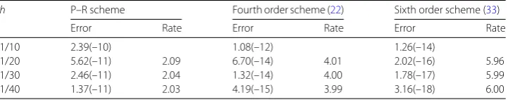
Table 3 L2-error and convergence rate for Problem1withτ= 0.001 atT= 1

1/10 2.39(–10) 1.08(–12) 1.26(–14)

1/20 5.62(–11) 2.09 6.70(–14) 4.01 2.02(–16) 5.96

1/30 2.46(–11) 2.04 1.32(–14) 4.00 1.78(–17) 5.99

1/40 1.37(–11) 2.03 4.19(–15) 3.99 3.16(–18) 6.00

To verify the accuracy in time, we ﬁx spatial grid sizeh= 0.02 and decrease the temporal sizes from 1/10 to 1/40 in Table2. It shows that scheme (22) and scheme (33) achieve the expected fourth order and sixth order accuracy in time, respectively. Table3shows theL2

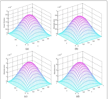
-norm error atT= 1 when we ﬁx temporal grid sizeτ = 0.001 and decrease the spatial grid sizes from 1/10 to 1/40. The results in Table3conﬁrm that scheme (22) and scheme (33) are fourth order and sixth order accuracy in space, respectively. These computed results are in full agreement with the theoretical accuracy order. Figure1depicts the absolute error obtained from scheme (22) and scheme (33) withh=τ = 1/20 atT= 1. It indicates that the present schemes indeed achieve a very high accuracy on comparably coarse mesh, as compared to conventional P–R splitting methods.

Problem 2

∂u ∂t =

1 17π2

∂2u ∂x2 +

∂2u ∂y2

, 0≤x,y≤4,t> 0.

The exact solution of this problem is

u(x,y,t) =e–tsin(4πx)sin(πy).

We design this problem to let the solutionuchange much faster inxdirection than iny

(13)

Figure 1The exact solution (a), the absolute error obtained from P–R scheme (b), present fourth order scheme (c), and present sixth order scheme (d), withh=τ= 1/20 atT= 1, Problem1

Table 4 L2_{-norm error and convergence rate for Problem}₂_with_h₌_τ_at_T_{= 1}

1/10 1.08(–2) 7.36(–3) 1.31(–3)

1/20 1.08(–2) 0.00 4.57(–4) 4.01 2.15(–5) 5.92

1/30 5.03(–3) 1.88 8.95(–5) 4.02 1.91(–6) 5.97

1/40 2.84(–3) 1.99 2.82(–5) 4.01 3.40(–7) 5.99

Table 5 L2-norm error for Problem2withτ= 0.2 atT= 1

h r=τ/h P–R scheme Fourth order scheme (22) Sixth order scheme (33)

Error Error Error

1/40 8 1.85(–3) 2.94(–5) 3.39(–7)

1/80 16 3.07(–4) 2.97(–6) 5.02(–9)

1/160 32 8.47(–4) 1.32(–7) 1.46(–10)

(14)

Figure 2The exact solution (a), the absolute error obtained from P–R scheme (b), present fourth order scheme (c), and present sixth order scheme (d), withh=τ= 1/20 atT= 1, Problem2

are plotted in Fig.2for Problem2. It shows that our splitting methods can still produce very accurate solution via signiﬁcantly coarse grid in the situation bypassing the accuracy barrier successfully.

5 Conclusion

(15)

schemes. It is worthy of being pointed out that the present methods can be straightfor-wardly extended to the three, or more, dimensional linear parabolic equations. Higher order and stable splitting methods can also be constructed in similar ways. We plan to report results from forthcoming research in this aspect in the near future.

Appendix

A sixth order finite difference for the one-dimensional steady diffusion equation

∂2_u

∂x2 =f(x), 0 <x< 1

with the boundary condition

u(0) =α, u(1) =β.

Leth=_N1 denote the step size of space, and deﬁnexi=ih,i= 0, 1, 2, . . . ,N. Based on Tay-lor’s series expansion of continuous functions, we get

f(xi)h2=

At the grid point 1, the sixth order formula is expressed as follows:

(16)

Similarly, we can construct the sixth order formula at grid pointN– 1:

uN–2– 2uN–1+uN

h2 =

3 32fN–

121 150fN–1+

127 1200fN–2–

1 150fN–3

+ 1 2400fN–4–

h2

200f

₍_xN_{) +}_O_h6_.

We can see more details in Ref. [2]. For the sake of completeness, we repeated the above deduction here.

Funding

This work has been partially supported by the National Natural Science Foundation of China under Grant 11772165, the National Natural Science Foundation of Ningxia under Grant 2018AAC02003, and the Key Research and Development Program of Ningxia under Grant 2018BEE03007.

Availability of data and materials

Not applicable.

Competing interests

The authors declare that they have no competing interests.

Authors’ contributions

JC deduced the two high order diﬀerence schemes in this paper, analyzed their stability and convergence, and conducted the numerical experiments. YG presented the idea of this work and wrote this manuscript. All authors read and approved the ﬁnal manuscript.

Authors’ information

Not applicable.

Publisher’s Note

Springer Nature remains neutral with regard to jurisdictional claims in published maps and institutional aﬃliations.

Received: 19 July 2018 Accepted: 30 September 2018 References

1. Sun, H.W., Zhang, J.: A high-order compact boundary value method for solving one-dimensional heat equations. Numer. Methods Partial Diﬀer. Equ.9, 846–857 (2003)

2. Lin, Y.X., Gao, J., Xiao, M.Q.: A high-order finite difference method for 1D nonhomogeneous heat equation. Numer. Methods Partial Differ. Equ.25, 327–346 (2009)

3. Zhao, J., Dai, W., Niu, T.C.: Fourth order compact schemes of a heat conduction problem with Neumann boundary conditions. Numer. Methods Partial Diﬀer. Equ.23, 949–959 (2007)

4. Li, J., Chen, Y., Liu, G.: High order compact ADI methods for parabolic equations. Comput. Math. Appl.52, 1343–1356 (2006)

5. Bialecki, B., De Frutos, J.: ADI spectral collocation methods for parabolic problems. J. Comput. Phys.229, 5182–5193 (2010)

6. Zhou, H., Wu, Y.J., Tian, W.: Extrapolation algorithm of compact ADI approximation for two-dimensional parabolic equations. Appl. Math. Comput.219, 2875–2884 (2012)

7. Qin, J.: The new alternating direction implicit diﬀerence methods for solving three-dimensional parabolic equations. Appl. Math. Model.34, 890–897 (2010)

8. Wang, Y.M.: Error and extrapolation of a compact LOD method for parabolic diﬀerential equations. J. Comput. Appl. Math.235, 1367–1382 (2011)

9. Wang, T., Wang, Y.M.: A higher-order compact LOD method and its extrapolations for nonhomogeneous parabolic diﬀerential equations. Appl. Math. Comput.237, 512–530 (2014)

10. Wang, T.: Alternating direction finite volume element methods for 2D parabolic partial difference differential equations. Numer. Methods Partial Differ. Equ.24, 24–40 (2008)

11. Peaceman, D.W., Rachford, H.H.: The numerical solution of parabolic and elliptic diﬀerential equation. J. Soc. Ind. Appl. Math.3, 28–41 (1955)

12. Dehghan, M.: A new ADI technique for two-dimensional parabolic equation with an integral condition. Comput. Math. Appl.43, 1477–1488 (2002)

13. Daoud, D.S.: On the numerical solution of multi-dimensional parabolic problem by the additive splitting up method. Appl. Math. Comput.162, 197–210 (2005)

14. Douglas, J., Kimy, S.: Improved accuracy for locally one-dimensional methods for parabolic equations. Math. Models Methods Appl. Sci.11, 1563–1579 (2001)

15. Dai, W., Nasar, R.: Compact finite difference scheme for solving parabolic differential equations. Numer. Methods Partial Differ. Equ.18, 129–141 (2002)

(17)

17. Zhao, J., Dai, W.Z., Zhang, S.Y.: Fourth order compact schemes for solving multi-dimensional heat conduction problems with Neumann boundary conditions. Numer. Methods Partial Diﬀer. Equ.24, 165–178 (2008)

18. Hiroaki, N.: First-, second-, and third-order ﬁnite-volume schemes for diﬀusion. J. Comput. Phys.256, 791–805 (2014) 19. Vu, T.L., Alexander, O.: Explicit exponential Runge–Kutta methods of high order for parabolic problems. J. Comput.

Appl. Math.259, 262–361 (2014)

20. Gao, F., Chi, C.M.: Unconditionally stable diﬀerence schemes for a one-space-dimensional linear hyperbolic equation. Appl. Math. Comput.187, 1272–1276 (2007)

21. Liu, H.W., Liu, L.B., Chen, Y.P.: A semi-discretization method based on quartic splines for solving one-space-dimensional hyperbolic equations. Appl. Math. Comput.210, 508–514 (2009)

22. Piao, X.F., Choi, H., Kim, S.D.: A fast singly diagonally implicit Runge–Kutta method for solving 1D unsteady convection-diﬀusion equations. Numer. Methods Partial Diﬀer. Equ.30, 788–812 (2013)

23. Zhang, Y.X.: [3, 3] Padé approximation method for solving space fractional Fokker–Planck equations. Appl. Math. Lett.

35, 109–114 (2014)

24. Hao, W., Zhu, S.: Domain decomposition schemes with high-order accuracy and unconditional stability. Appl. Math. Comput.219, 6170–6181 (2013)

25. Liu, D., Kuang, W., Tangborn, A.: High-order compact implicit diﬀerence methods for parabolic equations in geodynamo simulation. Adv. Math. Phys.2009, Article ID 568296 (2009).https://doi.org/10.1155/2009/568296

26. Liu, D., Chen, Q., Wang, Y.: A sixth order accuracy solution to a system of nonlinear diﬀerential equations with coupled compact method. J. Comput. Eng.2013, Article ID 432192 (2013).https://doi.org/10.1155/2013/432192

27. Sheng, Q.: Solving linear partial differential equations by exponential splitting. IMA J. Numer. Anal.9, 199–212 (1989) 28. Hirsh, R.S.: High order accurate difference solutions of fluid mechanics problem by a compact differencing

technique. J. Comput. Phys.19, 90–109 (1975)

29. Cuyt, A.: Padé Approximants for Operators: Theory and Applications. Lecture Notes in Mathematics. Springer, Berlin (1984)