R E S E A R C H
Open Access
A mass conserved splitting method for the
nonlinear Schrödinger equation
Dong-Ying Hua
1, Xiang-Gui Li
1*and Jiang Zhu
2* Correspondence: xianggui-li@vip. sina.com
1School of Applied Science, Beijing
Information Science and Technology University, Beijing 100192, P. R. China
Full list of author information is available at the end of the article
Abstract
A mass conserved time-splitting difference method is presented for the one-dimensional dipolar Bose-Einstein condensates (BECs) described by a nonlocal nonlinear Schrödinger equation with a convolution term. As a result of the
singularity in the convolution term, it brings difficulties both in mathematical analysis and in numerical simulations. By properly using the difference scheme to deal with the convolution term, an imaginary time method is given to compute the ground states and then a time-splitting method is obtained for dynamics of dipolar BECs. This time-splitting numerical method is mass conserved everywhere, and it has second-order accuracy and is also unconditionally stable. Numerical results are given to verify the stability and energy conservation when there is no blow up.
Mathematics Subject Classification (2010)65M06; 35Q41.
Keywords:time-splitting, finite difference, dipolar Bose-Einstein condensates,
Schrödinger equation, conservation
1 Introduction
Since its first experimental realization in dilute bosonic atomic gases in 1995, the Bose-Einstein condensation (BEC) of ultra-cold atomic and molecular gases has attracted considerable interests both theoretically and experimentally. Most of their properties of these trapped quantum gases are governed by the interactions between particles in the condensate [1]. In recent years, there has been an investigation for realizing a new kind of quantum gases with the dipolar interaction, acting between particles having a permanent magnetic or electric dipole moment. A BEC of52Cr atoms was realized [2,3] at Stuttgart University in 2005, which paves the way towards the experimental as well as the theoretical and the numerical investigation on this novel dipolar quantum gases. The interest on dipolar gases has also been motivated by a broad range of excit-ing applications [4-6]. In such condensates, there are two kinds of interactions, namely, the short-range repulsive interaction between the particles as well as their long-range partially attractive/partially repulsive dipolar interactions. Therefore, the macroscopic condensate dynamics is determined by a dynamical equilibration of these forces [7,8]. The effects of the interparticle interactions on the condensate properties have been widely discussed for the case of short-range interactions. However, since the dipole-dipole interactions are long range, anisotropic and partially attractive, the nontrivial task of achieving and controlling dipolar BECs is thus particularly challenging.
As we know, the properties of a BEC at temperaturesT very much smaller than the critical temperatureTcare usually described by the nonlinear Schrödinger (NLS) equa-tion for the macroscopic wave funcequa-tion known as the Gross-Pitaevskii (GP) equaequa-tion. As far as the dipolar interaction is concerned, a convolution term is introduced [9-11] to modify the classical GP equation, which results in the following differential-integral equation
ih¯ψt(x,t) =
− ¯h 2m∇
2+V(x) +gψ(x,t)2
+Vdip(x)∗ψ(x,t)2
ψ(x,t), (1)
whereħis the Planck constant,mthe mass of the atom andV(x) is the external trap-ping potential, which is generally harmonic, andg= 4πħ2as/mis the local interactions between dipoles in the condensate withasthe s wave scattering length (positive for repul-sive interaction and negative for attractive interaction).Vdip(x) is the long-range isotropic dipolar interaction potential between two dipoles. The wave functionψ(x,t) is normalized according to
ψ2=
R3
ψ(x,t)2dx=N, (2)
where Nis the number of the atoms in the dipolar BEC. The Equation 1 can be made dimensionless and simplified by adopting a unit system where the units for length, time and energy are given bya0, 1/ω0, andħω0, respectively, withω0= min{ω1,
ω2,ω3}, a0=
¯ h
mω0. Here, we only consider the one-dimensional (1D) case. Apart from
a conceptual clarity, lower dimensional dipolar BECs also offer a clear advantage for numerical computations. And also, in the case of radial symmetry in 2D and spherical symmetry in 3D (by tuning the trap frequencies), the multi-dimensional problem can be reduced to 1D case.
Now consider the following 1D dimensionless GP equation:
i∂ψ(x,t) ∂t =
−1 2∇
2+V(x) +βψ(x, t)2
+λVdip(x)∗ψ(x,t)2
ψ(x,t), (3)
ψ(x, 0) =ψ0(x), x∈R, (4)
where tis time,x is displacement,b andl are two dimensionless real parameters stand for the strength of the short-range interaction between the particles and the long-range dipolar interaction, respectively. ψ(x, t) :R×R+→C is a complex-valued function, V(x) =x2/2 stands for the harmonic potential in 1D,Vdip(x) = |x|-a, 0 <a< 1 is the convolution kernel representing the dipolar potential and * is the stan-dard convolution in R, i.e.,
Vdip(x)∗ψ(x, t)2=
R
ψ(y,t)2
x−yα dy, x,y∈R. (5)
existence of standing waves was proven in [13,14]. Due to the dipolar interaction potential of the nonlocal NLS, mathematical and numerical difficulties are introduced. Currently, the Fourier transform [15,16] is generally used for dealing with the convolu-tion in (3). However, there are two limitaconvolu-tions in these numerical methods: (i) the Fourier transform of the dipolar interaction potentialVdip(x) and the density function is usually carried out in the whole space R in the continuous level, while they are car-ried out on a bounded domainΩin the discrete level, so there is a locking phenomena in practical computation as observed in [17]; (ii) the denominator of the dipolar inter-action potential equals zero when x equals y, thus this singularity may cause some numerical difficulties too. The purpose here is to present a robust method for comput-ing ground states and dynamics of dipolar BECs without these two limitations. The key issue is to deal with the convolution term in the nonlocal NLS equation efficiently. This paper is organized as follows. In Sect. 2, some analytic results are given for the nonlocal NLS. In Sect. 3, a Crank-Nicolson numerical method is presented for com-puting ground states of dipolar BECs. In Sect. 4, a time-splitting numerical scheme is proposed for computing the dynamics. Numerical results are reported to verify the effi-ciency of this numerical method in Sect. 5. Finally, some concluding remarks are drawn in Sect. 6.
2 Analytical results
Two important invariants of (3) are the mass (or normalization) of the wave function
N(ψ(x, t)) := ψ(x, t)2=
R
ψ(x, t)2dx≡
R
ψ(x, 0)2dx= 1, t≥0, (6)
and the energy of per particle
E(ψ(x,t)) : =
R
1 2|∇ψ|
2+V(x)|ψ|2+β
2|ψ|
4+λ
2(Vdip(x)∗ |ψ|
2)|ψ|2 dx
≡E(ψ(x, 0)), t≥0.
(7)
In order to obtain the ground states, we take the ansatz
ψ(x, t) = e−iμtφ(x), x∈R, t≥0, (8)
where μ∈R is the chemical potential andj:=j(x) is a time-independent function. Inserting (8) into (3), we get the time-independent GP equation or the eigenvalue pro-blem
μφ(x) = (−1 2∇
2+V(x) +βφ(x)2
+ λVdip(x)∗φ(x)2)φ(x), x∈R, (9)
under the constraint
φ :=
R
φ(x)2dx= 1. (10)
Find jgÎSand μg∈R such that
Eg:=E(φg) = min
φ∈S E(φ), μ g:=μ(φ
g), (11)
where the nonconvex setSis defined as
S:={φ(x)| φ= 1, E(φ)<∞}. (12)
And the chemical potential (or eigenvalue of (9)) is defined as
μ(φ) : =
R
{1 2|∇φ|
2+V(x)|φ|2+β|φ|4+λ(V
dip(x)∗ |φ|2)|φ|2}dx
≡E(φ) +1 2
R
{β|φ|4+λ(V
dip(x)∗ |φ|2)|φ|2}dx.
(13)
The total energy in (7) is composed of kinetic, potential, interaction and dipolar energies, respectively, i.e.,
E(φ) =Ekin(φ) +Epot(φ) +Eint(φ) +Edip(φ), (14)
where
Ekin(φ) =
1 2
R
|∇φ|2dx, E pot(φ) =
R
V(x)|φ(x)|2dx,
Eint(φ) = β
2
R
|φ(x)|4dx, Edip(φ) = λ
2
R
(Vdip(x)∗ |φ(x)|2)|φ|2dx,
and j(x) defined in (8) is a stationary state of a dipolar BEC.
3 Numerical method for computing ground states
In this section, we will propose an implicit numerical method for computing the ground states of a dipolar BEC. In practical computation, we usually truncate the problem (3) and (4) into a bounded computational domainΩ(chosen as an interval [−a,a] in 1D, withasufficiently large), with homogeneous Dirichlet boundary condition. There are various numerical methods proposed in literatures for computing the ground states of BEC [8,9,16-19]. One of the efficient and popular techniques for the constraint (6) is through the following construction [13]: we choose a time step sizeτ> 0 and settk=kτ fork= 0, 1,. ... Applying the imaginary time method [18] without considering the con-straint (6), and then projecting the solution back to the unit nonconvex setSat the end of each time interval [tk, tk+1] to satisfy the constraint. Then the functionj(x, t) is the solution of the following gradient flow with discrete normalization [19]:
∂φ(x,t) ∂t =
1 2∇
2−V(x)−β|φ(x, t)|2−λV
dip(x) ∗ |φ(x, t)|2 φ(x, t), (15)
φ(x, t)|x∈∂ = 0, t≥0, (16)
φ(x, tk+1) :=φ(x, t+k+1) =
φ(x,t−k+1)
φ(x, 0) =φ0(x), φ0= 1, (18)
where φ(x, t±k) = limt→tk±φ(x, t) and j0(x) is the initial condition.
SupposeMis a positive integer, choose the spatial steph= 2a/M, and define xj=−a
+j h, j= 0, 1,. .. , M. Let Fk
j be the approximation ofVdip(xj) *|j(xj, tk)|2, and φjk be
the approximations of (xj, tk), which are the exact solution of (15)-(18) at the mesh grid (xj, tk).
Choose φ0j =φ0(xj),j= 0, 1,. .. ,M. From timetktotk+1, a cental difference
discre-tization for (15)-(18) is
φk+1 j −φjk
τ =
1 2h2δ
2 x(φ
k+1/2
j )−V(xj)φjk+1/2−β(|φkj|2)φ k+1/2 j −λFkjφ
k+1/2
j , j= 0, 1,. . .,M, (19)
where
φk+1/2
j = (φjk+1+φjk)/2, δ2x(φjk) =φkj+1−2φjk+φjk−1,
Fk j=
M−1
r=0
1
1−α|φ(xr,tk)|
2||(r+ 1−j)h|1−α− |(r−j)h|1−α|+|φ(xr+1,tk)|2− |φ(xr−1,tk)|2
2h .
h
0 s
|(r−j)h+s|αds+|φ
(xr+1,tk)|2−2|φ(xr,tk)|2+|φ(xr−1,tk)|2
h2 ·
h
0 s2 2|(r−j)h+s|αds
⎞ ⎠,
(20)
and the details of Fjkare given in the Appendix. Notice that in the above scheme, we
replace β(|φjk+1/2|2)φk+1/2
j , F
k+1/2
j with β(|φjk|2)φ k+1/2
j andFj
k, respectively, to linearize
the nonlinear terms. It is easy to see that the local truncation error of (19) is O(h2 +τ 2
) because 0 <a< 1. Using the classical finite difference method theory, we claim our numerical scheme is the second-order algorithm which will be justified by the numeri-cal examples in Sect. 5.
4 Time-splitting numerical method for dynamics
We will propose a time-splitting finite difference (TSFD) method for computing the dynamics of a dipolar BEC based on the nonlocal NLS equation (3). The advantage of this method is to deal with the discretization of nonlinear terms in the NLS equation by solving an ordinary differential equation (ODE) exactly. By virtue of this way, the computational cost and complexity can be reduced. As in Sect. 3, the whole space pro-blem is truncated into a bounded computational domain Ω= [−a, a] with homoge-neous Dirichlet boundary condition.
From t=tkto t=tk+1, the GP equation (3)-(4) is solved by three steps. First, we solve
i∂ψ(x,t) ∂t =−
1 2∇
2ψ(x, t), x∈ , (21)
ψ(−a, t) = 0, ψ(a, t) = 0, (22)
fromtktotk+1/2, followed by solving the nonlinear ODE
i∂ψ(x,t)
∂t = (V(x) +β|ψ(x, t)|
2+λV
ψ(−a, t) = 0,ψ(a, t) = 0,tk≤t≤tk+1, (24)
for one time step. Again, we slove (21) fromtk+1/2totk+1.
Equation 21 can be discretized in space by Crank-Nicolson scheme, and Equation 23 can be solved exactly. In fact, for tÎ[tk, tk+1], multiplying (23) by the conjugation of ψ(x, t), i.e., ψ(x,t), we get
i∂ψ(x,t)
∂t ψ(x,t) =
V(x) +β|ψ(x, t)|2+λVdip(x)∗ |ψ(x, t)|2
ψ(x, t)ψ(x,t),(25)
and we also have
−i∂ψ(x,t)
∂t ψ(x, t) =
V(x) +β|ψ(x, t)|2+λVdip(x)∗ |ψ(x, t)|2
ψ(x,t)ψ(x, t), (26)
Therefore, subtracting (26) from (25), one obtains
id
dt|ψ(x, t)|
2 = 0.
which implies
|ψ(x, t)|2= |ψ(x, tk)|2, tk≤t≤tk+1. (27)
Substituting (27) into (23), we get a linear ODE
i∂ψ(x,t)
∂t = (V(x) +β|ψ(x, tk)|
2+λV
dip(x)∗ |ψ(x, tk)|2)ψ(x, t) (28)
which can be solved exactly. Integrating (28) fromtktot, one gets
ψ(x,t) = exp{−i[V(x)+β|ψ(x, tk)|2+λVdip(x)∗|ψ(x, tk)|2](t−tk)}ψ(x, tk), tk≤t≤tk+1. (29)
Let ψjkbe the approximation ofψ(xj, tk). Then a second-order TSFD method for sol-ving (3)-(4) via the standard Strang splitting [20-22] is as follows:
⎧ ⎪ ⎨ ⎪ ⎩
ψ(1)
j−1+ (4i/λ0−2)ψj(1)+ψ (1)
j+1 =−ψjk−1+ (4i/λ0+ 2)ψjk−ψjk+1,
ψ(2)
j = exp{−iτ[V(xj) +β|ψ (1) j |2+λF
(1) j ]}ψ
(1)
j , j= 1, 2, . . ., M−1,
ψk+1
j−1+ (4i/λ0−2)ψjk+1+ψjk+1+1=−ψ (2)
j−1+ (4i/λ0+ 2)ψj(2)−ψ (2) j+1,
(30)
wherel0=τ/2h2,ψM= 0 and F (1)
j =Vdip(xj) ∗ |ψ (1) j |2.
The above method is implicit, unconditionally stable. In fact, for the stability or con-servation, we have
Theorem 1.The scheme (30) is normalization conservation, i.e.,
ψk+12
l2 :=h M
j=0 |ψk+1
j |2≡h M
j=0 |ψ0
j|2=ψ0 2
l2, k≥0. (31)
Proof. According to the first equation of (30), if we denote Aj=ψj(1)+ψjk, we have
4i λ0
Multiplying (32) by the conjugation of Aj, one gets
Combine the above two equations, we have
8i to see that, the right-hand side vanishes due to the homogeneous Dirichlet boundary conditionψ0 =ψM= 0.
Therefore, we have the following equation
M−1
Similarly, the following equation is obtained from the third equation of (30),
M−1
Based on Equation (29) and the second equation of (30), we have
M−1
Combining (35), (36) with (37), we have
M−1
In this section, we first evaluate numerically the convolution term and then report ground states and dynamics of dipolar BECs using our numerical method.
5.1 Error for the convolution term
the third-order accuracy. We choosea= 0.5 and solve this problem on [0, 10]. Table 1 shows the maximum errors with different sizes h.
From Table 1, one can see that our new method has a higher order accuracy between the second-order and the third-order in space for evaluating the convolution term.
5.2 Ground states of dipolar BECs
Using numerical scheme (15)-(18), the ground states of a dipolar BEC with different
parameters are given. The initial condition is φ0(x) = π11/4e− x2/2
. We solve this problem
on [−16, 16] withh= 1/8 andτ= 0.001.jg:=jk+1is reached numerically when
φk+1−φk
∞ := max0≤j≤M|φ k+1
j −φkj| ≤ ε:= 10−6
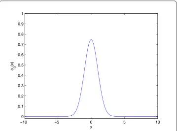
in (15). Figure 1 shows the plot of the ground statejg(x), of a dipolar BEC withl= −0.2 and b= 0.5. Table 2 shows the energyEg, chemical potentialµg, kinetic energy
Egkin:=Ekin(φg), potential energy Egpot:=Epot(φg), interaction energy Egint :=Eint (φg),
dipolar energy Egdip:=Edip(φg), and the maximum value of the wave function jg(0)
with a= 0.5 and potentialV (x) =x2/2 for different l andb with fixedl/b=−0.4; Table 3 gives computational results with b= 0.5 for different values of −0.5≤l/b≤1. In addition, since the GP equation has no analytical solution, we take the numerical solution in a finer mesh withM = 2048 andτ= 0.001 as the“exact” solution, and the maximum error are given in Table 4.
From Tables 2, 3, 4, and Figure 1, we make the following conclusions: when l increases or bdecreases with fixedl/b=−0.4, the maximum value of the wave
func-tion jg(0), kinetic energy Egkin, dipolar energy Egdip, energy Egas well as the chemical
potential µgincrease; the potential energy Egpot, interaction energy Egint, and the radius
mean square xgrms, defined by xrms=
R
x2|φ
g(x)|2dx decrease (cf. Table 2). For fixed
b , when the ratio l/b increases from −0.5 to 1, Egpot,E g
dip, Eg µg , andxrms of the
ground states increase; the maximum value of the wave functionjg(0), Egkin, and Egint
decrease (cf. Table 3). This numerical method is second-order accurate and can com-pute the ground states efficiently (cf. Figure 1; Table 4).
5.3 Dynamics of dipolar BECs
By applying our numerical method (30), the dynamics of a dipolar BEC is considered. We apply the bounded computational domain [−8, 8],M = 128, i.e.,h= 1/8, time step τ = 0.01. The initial data is chosen the same as in the case of computing the ground state of a dipolar BEC.
Table 1 Comparison for evaluating the convolution term under varying spatial sizesh
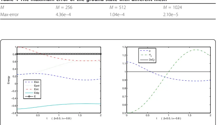
Figure 2 depicts the evolution of kinetic energy Ekin(t):= Ekin(ψ(·, t)), potential energy
Epot(t):= Epot(ψ(·, t)), interaction energyEint(t):=Eint(ψ(·, t)), dipolar energyEdip(t):= Edip (ψ(·, t)), the energyE(t):=E(ψ(·, t)) as well as the chemical potentialµ(t) := µ(ψ(·, t)),
condensate width σx:=σx(ψ(·, t)) =
R
x2|ψ(x, t)|2dx
, andl2 normψ(·, t)l2 for the
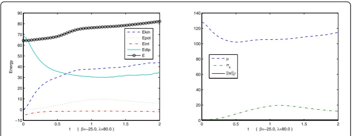
case of b= 5.0 and l=−0.8. In addition, Figure 3 shows the results for the case of b= 25 andl= 0.8. Figure 4 shows the results for the case ofb=−25 andl= 80.
From Figures 2, 3, and 4, we can obtain the conclusion that global existence of the solution is observed in the first two cases (cf. Figures 2, 3) and finite time blow-up is observed in the last case (cf. Figure 4). The total energy is numerically conserved in our computation when there is no blow-up (cf. Figures 2, 3) and the discrete l2 -norm ||ψ|| is numerically conserved very well whether there is blow-up or not (cf. Figures 2, 3, 4).
−10 −5 0 5 10
0 0.1 0.2 0.3 0.4 0.5 0.6 0.7 0.8 0.9 1
x g
(x)
Figure 1The ground state of a dipolar BEC withl=−0.2 andb= 0.5.
Table 2 The ground states of a dipolar BEC for differentlandbwith fixed values of
l/b=−0.4.
l,b jg(0) Egkim Egpot E
g
int E
g
dip E
g
μg
xgrms
l=−0.2,b= 0.5 0.747990 0.247231 0.252333 0.099135 −0.171511 0.427188 0.354812 0.710398
l=−0.1,b= 0.25 0.749946 0.248765 0.250757 0.049763 −0.085918 0.463367 0.427212 0.708176
l=−0.02,b= 0.05 0.751125 0.249513 0.250000 0.009974 −0.017201 0.492285 0.485058 0.707106
l= 0.02,b=−0.05 0.751581 0.249878 0.249634 −0.009983 0.017208 0.506737 0.513963 0.706589
l= 0.1,b=−0.25 0.753250 0.251210 0.248312 −0.050082 0.086181 0.535622 0.571721 0.704716
6 Conclusions
Efficient numerical methods are presented for computing ground states and dynamics of dipolar Bose-Einstein condensates based on the one-dimensional Grosss-Pitaevskii equation with a nonlocal dipolar interaction potential. By applying the difference Table 3 The ground states of a dipolar BEC with different values ofl/bforb= 0.5
l/b jg(0) Egkim Egpot Egint E
g
dip E
g
μg
xgrms
−0.5 0.751923 0.251344 0.248178 0.100052 −0.215360 0.384214 0.268906 0.704526
−0.2 0.738615 0.237322 0.262981 0.096925 −0.084809 0.512420 0.524537 0.725233 0 0.729516 0.228042 0.273869 0.094808 0.000000 0.596719 0.691527 0.740093 0.2 0.720684 0.219377 0.284956 0.092781 0.083002 0.680116 0.855899 0.754926 0.5 0.707932 0.207437 0.301936 0.089903 0.204307 0.803583 1.097793 0.777092 1 0.688010 0.190073 0.330997 0.085519 0.398668 1.005257 1.489444 0.813631
Table 4 The maximum error of the ground state with different mesh
M M= 256 M= 512 M= 1024
Max-error 4.36e−4 1.04e−4 2.10e−5
0 0.5 1 1.5 2
−0.8
−0.6
−0.4
−0.2
0 0.2 0.4 0.6 0.8 1
t (=5.0,=−0.8 )
Energy Ekin
Epot Eint Edip E
0 0.5 1 1.5 2
0.5 0.6 0.7 0.8 0.9 1 1.1 1.2 1.3
t (=5.0,=−0.8 )
x
|||| l2
Figure 2Time evolution at different times for a dipolar BEC withb= 5.0 andl=−0.8.
0 0.5 1 1.5 2
0 1 2 3 4 5 6 7
t (=25.0,=0.8 )
Energy
Ekin Epot Eint Edip E
0 0.5 1 1.5 2
0 2 4 6 8 10 12
t (=25.0,=0.8 )
x
||||l2
method, the discretization of the dipolar interaction potential term is given. The ima-ginary method and time-splitting difference method are given for computing the ground states and dynamics of a dipolar BEC, respectively. Our numerical method is mass conserved and second-order accurate. In addition, the proof of the discrete energy conservation is an open problem. We only find the energy conservation from a numerical point of view. Numerical results are given to demonstrate the efficiency of our numerical method.
Appendix
The discretization of the convolution term Here, we need to handle the convolution term
Vdip(x) ∗ |ψ(x, t)|2= |x|−α∗ |ψ|2= zised integration area. It is easy to see that xjis a singular point and we need to deal
Then, substituting|j(xr+s, tk)|2by the Taylor expansion at (xr, tk), we obtain
Combining (A.1), (A.3) and (A.4), we obtain the discretization of convolution term
Fkj =
Acknowledgements
This work was supported by National Natural Science Foundation of China (No. 11171032) and Beijing Municipal Education Commission (Nos. KM201110772017, 71D09111003).
Author details
1School of Applied Science, Beijing Information Science and Technology University, Beijing 100192, P. R. China 2National Laboratory for Scientific Computing, Ministry of Science and Technology, Avenida Getulio Vargas 333,
25651-075 Petropólis, RJ, Brazil
Authors’contributions
DY H established the scheme, performed the numerical examples in section 5.1, 5.2 and drafted the manuscript. XG L designed the study and carried out the the numerical simulations in section 5.3. J Z participated in explaining the physical background, established the model and helped to inspect the manuscript. All authors read and approved the final manuscript.
Competing interests
The authors declare that they have no competing interests.
Received: 22 April 2012 Accepted: 21 June 2012 Published: 21 June 2012
References
1. Pitaevskii, L, Stringari, S: Bose-Einstein Condensation. Oxford University, New York (2003)
2. Griesmaier, A, Werner, J, Hensler, S, Stuhler, J, Pfau, T: Bose-Einstein condensation of chromium. Phys Rev Lett94(2005). article 160401
3. Stuhler, J, Griesmaier, A, Koch, T, Fattori, M, Pfau, T, Giovanazzi, S, Pedri, P, Santos, L: Observation of dipole-dipole interaction in a degenerate quantum gas. Phys Rev Lett.95, article 150406 (2005)
4. Baranov, MA, Mar’enko, MS, Rychkov, VS, Shlyapnikov, GV: Superfluid pairing in a polarized dipolar Fermi gas. Phys Rev A66(2002). article 013606
5. Góral, K, Santos, L, Lewenstein, M: Quantum phases of dipolar bosons in optical lattices. Phys Rev Lett88(2002). article 170406
6. Kawaguchi, Y, Saito, H, Ueda, M: Einstein-de Haas effect in dipolar Bose-Einstein condensates. Phys Rev Lett96(2006). article 080405
7. Lahaye, T, Menotti, C, Santos, L, Lewenstein, M, Pfau, T: The physics of dipolar bosonic quantum gases. Rep Prog Phys 72(2009). article 126401
8. Santos, L, Shlyapnikov, GV, Zoller, P, Lewenstein, M: Bose-Einstein condensation in trapped dipolar gases. Phys Rev Lett. 85, 1791–1794 (2000). doi:10.1103/PhysRevLett.85.1791
9. Yi, S, You, L: Trapped atomic condensates with anisotropic interactions. Phys Rev A61(2000). article 041604(R) 10. Yi, S, You, L: Trapped condensates of atoms with dipole interactions. Phys Rev A63(2001). article 053607 11. Yi, S, You, L: Calibrating dipolar interaction in an atomic condensate. Phys Rev Lett92(2004). article 193201 12. Carles, R, Markowich, PA, Sparber, C: On the Gross-Pitaevskii equation for trapped dipolar quantum gases. Nonlinearity.
21, 2569–2590 (2008). doi:10.1088/0951-7715/21/11/006
13. Bao, W, Cai, Y, Wang, H: Efficient numerical methods for computing ground states and dynamics of dipolar Bose-Einstein condensates. J Comput Phys.229, 7874–7892 (2010). doi:10.1016/j.jcp.2010.07.001
14. Chen, J, Guo, B: Strong instability of standing waves for a nonlocal Schrödinger equation. Physica D.227, 142–148 (2007). doi:10.1016/j.physd.2007.01.004
15. Lahaye, T, Metz, J, Fröhlich, B, Koch, T, Meister, M, Griesmaier, A, Pfau, T, Saito, H, Kawaguchi, Y, Ueda, M:d-Wave collapse and explosion of a dipolar Bose-Einstein condensate. Phys Rev Lett101(2008). article 080401
16. Góral, K, Rzążewski, K, Pfau, T: Bose-Einstein condensation with magnetic dipole-dipole forces. Phys Rev A.61, article 051601(R) (2000)
17. Ronen, S, Bortolotti, D, Bohn, J: Bogoliubov modes of a dipolar condensate in acylindrical trap. Phys Rev A74(2006). article 013623
18. Chiofalo, ML, Succi, S, Tosi, MP: Ground state of trapped interacting Bose-Einstein condensates by an explicit imaginary-time algorithm. Phys Rev E.62, 7438–7444 (2000). doi:10.1103/PhysRevE.62.7438
19. Bao, W, Du, Q: Computing the ground state solution of Bose-Einstein condensates by a normalized gradinet flow. SIAM J Sci Comput.25, 1674–1697 (2004). doi:10.1137/S1064827503422956
20. Strang, G: On the construction and comparison of difference schemes. SIAM J Numer Anal.5, 505–517 (1986) 21. Li, XG, Chan, CK, Hou, Y: A numerical method with particle conservation for the Maxwell-Dirac system. Appl Math
Comput.216, 1096–1108 (2010). doi:10.1016/j.amc.2010.02.002
22. Bao, W, Li, XG: An efficient and stable numerical method for the Maxwell-Dirac system. J Comput Phys.199, 663–687 (2004). doi:10.1016/j.jcp.2004.03.003
doi:10.1186/1687-1847-2012-85