Earth Planets Space,50, 635–640, 1998
Improving geomagnetic field models for the period 1980–1999 using Ørsted data
Pascale Ultr´e-Gu´erard, Dominique Jault, Mioara Alexandrescu, and Jos´e Achache
Institut de Physique du Globe de Paris, 4 Place Jussieu, 75252 Paris Cedex 05, France (Received October 9, 1997; Revised February 2, 1998; Accepted May 11, 1998)
The Danish satellite Ørsted is due to be launched in 1998, and should provide, for the first time since the Magsat mission (1979–1980), a dense and global coverage of the Earth’s surface with vector measurements of the magnetic field. In this paper, we compare the expected error in the main field models computed for the 1970–1999 time interval using observatory data, with or without the a priori information given by the knowledge of the field at both Magsat and Ørsted epochs. This work is based on the reasonable hypothesis that the main field models derived from Ørsted data will be as accurate as the Magsat models. The a priori information given by the Magsat and Ørsted models is based on a linear behaviour of the rate-of-change of the field throughout this period, plus a noise level which can be estimated as a function of time and degree from past field changes. The expected error in the models computed for the 1980–1999 period with a priori information appears to be significantly smaller than the expected error in the models computed without this information. This result is related to the heterogeneous distribution of the observatories over the Earth surface. Consequently, when the Ørsted data is available, improved models can be computed for the 1980–1999 period particularly in regions without observatory data. This method with a priori information may allow the use of the same set of observatories throughout the entire period. Indeed, our method alleviates the requirement of a very dense data distribution.
1.
Introduction
Because of the heterogeneous distribution of observatories over the Earth’s surface, main field models are plagued with large errors as harmonical analysis degree and order values become larger when they are computed using only observa-tory data (Alexandrescuet al., 1994). Furthermore, Alexan-drescuet al.(1994) show that, even for the smallest degrees, these errors are large as indicated by the covariance matrices. Indeed, global field models can be computed applying Gauss potential field theory, but for regions with few observatories (i.e., the Pacific, Indian, and most of the Atlantic Oceans) the field is not accurately determined. The Magsat satel-lite, launched in November 1979, provided accurate vector measurements of the Earth’s magnetic field with a dense and homogeneous distribution. Thus, the main field has been accurately modelled for the 1980.0 epoch (e.g., Langel and Estes, 1985; Bloxhamet al., 1989; Cohen, 1989). Estimat-ing the crustal biases of the observatories has also enhanced the accuracy of main field models for other epochs (Langel et al., 1982; Gubbins and Bloxham, 1985; Langel and Estes, 1985; Bloxhamet al., 1989). However, the Magsat mission has given almost no information on the geomagnetic field SV (Secular Variation—the first time derivative of the field). Thanks to the Danish Ørsted satellite, which is scheduled to be launched in 1998, we may obtain for the first time since Magsat, a global and dense coverage of the Earth’s surface with accurate vector measurements of the magnetic field. This mission should be closely followed by other satellite
Copy right cThe Society of Geomagnetism and Earth, Planetary and Space Sciences (SGEPSS); The Seismological Society of Japan; The Volcanological Society of Japan; The Geodetic Society of Japan; The Japanese Society for Planetary Sciences.
missions such as CHAMP, SAC-C, Sunsat, Fedsat, DMSP Block 5, NPOESS over the coming years. Hopefully, it will be possible to compute accurate models of the field from 1999 onwards. Obviously, knowledge of the field at the epochs of Magsat and Ørsted will allow the computation of the linear component of the magnetic field time-variation between 1980 and 1999. In this study, we show that the simultaneous use of Magsat and Ørsted data will improve our knowledge of SV, as well as our knowledge of the higher frequencies of the time-variations of the geomagnetic field around the period 1980–1999.
2.
Method
2.1 Inverse problem
Our objective is to show how the knowledge of the geo-magnetic field at Magsat and Ørsted epochs (respectively 1980.0 and 1999.0) will improve the computed models using observatory data throughout the 1980–1999 period. In doing so, coherence between the different data sets is expected. The discrepancies in field values between Magsat models and observatory data have been attributed to local crustal field at the observatories. These biases are thought to stay constant with time. This is confirmed in a recent paper in which observatory data corrected with biases calculated during the Magsat epoch are shown to be compatible with data from the POGS satellite for the period 1991–1993 (Ultr´e-Gu´erard and Achache, 1997).
The method applied here is based on a least-squares in-version with a priori information (see e.g., Tarantola and Valette, 1982; Langel, 1987). A model is computed using the a priori information given by the linear time-variation of the field between Magsat and Ørsted. The inversion consists
636 P. ULTRE-GU´ ERARD´ ET AL.: IMPROVING GEOMAGNETIC FIELD MODELS FOR THE PERIOD 1980–1999
XComputedmodel −XObs
2
+WvecY
YComputedmodel −YObs
2
+WvecZ
ZmodelComputed−ZObs
2
(1)
wheretMagsatandtØrstedare the times of Magsat andØrsted
missions respectively,tModeldenotes the time for which the
model is calculated. Time can be before, between, or after the two missions. gMagsatmodel,gComputedmodel andgØmodelrsteddefine the Gauss coefficients of the models computed attMagsat,tModelandtØrsted
epochs respectively. gMagsat0 andg0Ørstedare the a priori models computed at Magsat andØrsted epochs, which give the linear trend of the rate-of-change between the Magsat andØrsted epochs. XComputedmodel ,YComputedmodel and ZComputedmodel are the compo-nents of thefield as computed by the modelgmodel
Computed. X Obs,
YObsandZObsare the 3 components of the geomagneticfield measured at the observatories. WMagsat,WComputed,WØrsted, WX
vec,W
Y
vec,W
Z
vecare the weights (see section below) applied
to the different terms. All the models are limited to degree and order 8 in order to compare our computed model with models derived from only observatory data. The coefficients of thefield at Magsat andØrsted epochs are unknown but the
weights entering thefirst and third terms on the right hand side of the equation are so large that these coefficients can be thought of as beingfixed. The model is constrained not to depart significantly from the linear trend given by Magsat andØrsted models in the second term of Eq. (1). Constraints given by the observatory measurements are incorporated in the fourth term. At the epoch tModel, the field is assumed
to be measured at 190 existing observatories. For compari-son, the inversion is also done for a hypothetical case where 190 ground data points are evenly distributed at the Earth’s surface.
2.2 Choice of the weights
Making the reasonable hypothesis that the models derived fromØrsted data will be as accurate as the models derived from Magsat data, the weights for Magsat andØrsted models (WMagsatandWØrsted) are taken to be equal and are estimated
for each Gauss coefficient as the inverse of the variance of the model computed with Magsat data. The weights for the observatory vector data are taken with respect to the value estimated by Langelet al.(1996), i.e.:
WvecC = 1
where theσvecare defined as the mean deviations of the
mea-sured components at the observatories from the values given by the model computed by Langelet al.(1996). These devi-ations do not include the crustal biases which are computed as unknown parameters during the inversion of the satellite and observatory data.
P. ULTRE-GU´ ERARD´ ET AL.: IMPROVING GEOMAGNETIC FIELD MODELS FOR THE PERIOD 1980–1999 637
Fig. 2. Deviationσ(see text) averaged for the 1900–1990 period versus the spherical harmonic degreenfor different time intervalst= −10,−5, 5, 10 and 15 yrs.
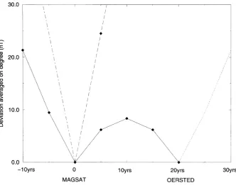
Fig. 3. Deviationσaveraged as a function of time (solid line). The deviation corresponding to Magsat proximity alone is given for comparison (dashed line). The dotted and dotted-dashed lines are symmetric about the computed lines.
the decade time-scale, can be described with a linear trend plus an estimated noise level. We checked that thisfirst order description is valid for periods including geomagnetic jerks of global extent (e.g., 1969, 1978). A more detailed study of those periods requires other approaches. The jerks can be expressed in the form of two second degree polynomials of
time with a sudden change in curvature at the time of the event (e.g., Courtillotet al., 1978; Achacheet al., 1980; Ducruix
638 P. ULTRE-GU´ ERARD´ ET AL.: IMPROVING GEOMAGNETIC FIELD MODELS FOR THE PERIOD 1980–1999
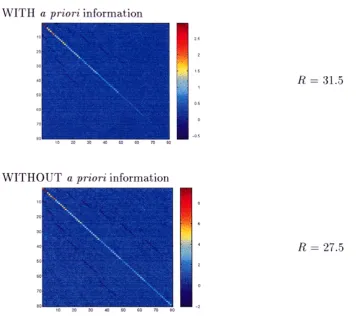
Fig. 4. Covariance matrices of the computed model obtained for an existing and uneven distribution of observatories, with and without the a priori information;g0
1is represented in the left upper part of each matrix, the degree and the order increases to the right and downwards. Units of the covariance
matrices are (nT)2. The ratioR(see text) is given in both cases.
P. ULTRE-GU´ ERARD´ ET AL.: IMPROVING GEOMAGNETIC FIELD MODELS FOR THE PERIOD 1980–1999 639
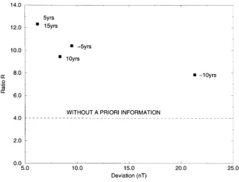
Fig. 6. Values of the ratioRas a function of the deviationσfor different time intervalst.
these approaches are not needed for our purpose. Our de-scription of the rate-of-change of thefield is also justified by the time constants of the geomagneticfield which are of the order of several hundred years for the axial dipole and of a couple of hundred years for the non-dipole terms (Hulot and Le Mouel, 1994). The discrepancy between an actual model¨
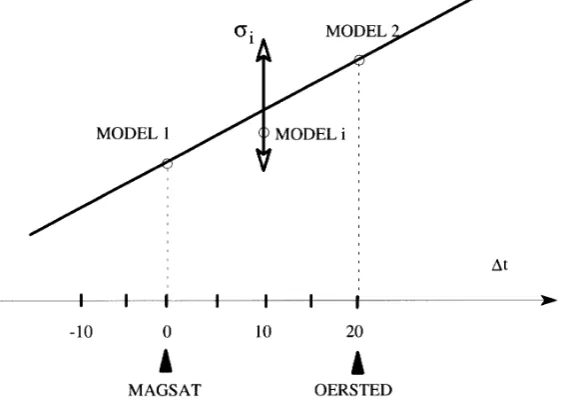
and a linearfit to two given end models 20 years apart is computed as a function of the degreenas follows:
σn = the chosen model (“model i”) from the linear interpolation between the coefficients of the two end models. It is calcu-lated as a function of the time interval between the epoch of the model and the epoch of thefirst assumed known model (t = −10,−5, 5, 10 and 15 years: see Fig. 1). The calcula-tion is performed for each set of two models, separated by 20 years, and the estimates are averaged for the period 1900–
1990. The calculated deviation is compared to the degree for the different time intervals in Fig. 2. Thisfigure shows that the deviation is greater for the negative values oft. Indeed,“model i”is outside of the interval between models 1 and 2 where the linear trend is defined. The deviation av-eraged over degree for different time intervalst is given in Fig. 3. Thisfigure also shows the deviation correspond-ing to the a priori information given by Magsat proximity alone, which supports the assumption of linear behaviour of the time-variations of thefield.
The covariance matrixATW A−1, whereAis the Jaco-bian matrix andW is the matrix of weights, associated with the computed model is estimated and compared with the ma-trix obtained when only observatory data are used without the
a priori information. For each matrix, the ratio between the quadratic mean of the diagonal terms and the quadratic mean of the non-diagonal termsR= (V)i i/(V)i jis also com-puted. Small values of R indicate large cross-correlations between the coefficients.
3.
Results
The inversion is performed in the case where the time-intervaltis equal to 10 years (this is the most unfavorable case for the time interval between Magsat andØrsted epochs, see Fig. 3).
Firstly, the covariance matrix of the computed model in the case of the actual observatory distribution is presented in Fig. 4. The covariance matrix, obtained when the observatory data are inverted without a priori information, is given for comparison. In this case, the ratio R is increased by the a priori information (from R=4 toR=9.5).
Secondly, the same matrices are computed for the hy-pothetical case of an even distribution of observatory data (Fig. 5). In this case, the improvement is shown to be less significant. Indeed, the variances are similar with or without the a priori information and the ratioRis not very different as it varies fromR=31.5 in thefirst case toR=27.5 in the second. These comparable values of Rdemonstrate that the a priori information obtained by the two sets of satellite data is so valuable given an uneven distribution of observatories. Finally, Fig. 6 gives the different values of the ratio R
640 P. ULTRE-GU´ ERARD´ ET AL.: IMPROVING GEOMAGNETIC FIELD MODELS FOR THE PERIOD 1980–1999
4.
Conclusion
The results of this study show a potential benefit to main
field modelling by using Ørsted data. When Ørsted data are available, we will compute annual models of the 1980–
1999 period, using the observatory data (annual means) and the mainfield models derived from Magsat andØrsted data. Their coefficients will be estimated with the a priori informa-tion given by the linear rate-of-change of thefield between Magsat andØrsted epochs using the method presented above. The present study also shows that the models computed with the a priori information will be more accurate than the exist-ing ones because of the uneven distribution of the observato-ries over the Earth’s surface. The knowledge of thefield in the regions where there is no ground data can be much improved. At the present time, referencefield models are computed by using data available from various origins (observatories, re-peat stations, surveys, aeromagnetic surveys,. . .) in order to have the best distribution at the Earth’s surface. Thanks to
Ørsted data and to the a priori information given by the lin-ear time-variation of thefield between Magsat andØrsted, it will be possible to compute accurate models with a carefully selected data set, composed only of the most accurate and continuous records of thefield. Indeed, if the data set is al-ways the same for every model, the error will be systematic and will cancel in secular variation models. We expect secu-lar variation models to be improved for a 40 year time interval around the Magsat andØrsted satellite missions and maybe for a longer period if current planned satellite missions are realised in the future.
Acknowledgments. We are pleased to thank the staff of the geo-magnetic observatories for their kind supplying of data. We would also like to thank the two referees, D. Barraclough and A. Jackson, for comments. This is IPGP contribution 1516.
References
Achache, J., V. Courtillot, J. Ducruix, and J.-L. Le Mouel, The late 1960¨ ’s secular variation impulse: further constraints on deep mantle conductiv-ity,Phys. Earth Planet. Inter.,23, 72–75, 1980.
Alexandrescu, M., C. Ha Duyen, and J. L. Le Mou¨el, Geographical distribu-tion of magnetic observatories andfield modelling,J. Geomag. Geoelectr.,
46, 891–901, 1994.
Alexandrescu, M., D. Gibert, G. Hulot, J.-L. Le Mou¨el, and G. Saracco, Detection of geomagnetic jerks using wavelet analysis,J. Geophys. Res.,
100, 12557–12572, 1995.
Alexandrescu, M., D. Gibert, G. Hulot, J.-L. Le Mou¨el, and G. Saracco, Wordwide wavelet analysis of geomagnetic jerks,J. Geophys. Res.,101, 21975–21994, 1996.
Bloxham, J. and A. Jackson, Time-dependent mapping of the magneticfield at the core-mantle boundary,J. Geophys. Res.,97, 19537–19563, 1992. Bloxham, J., D. Gubbins, and A. Jackson, Geomagnetic secular variation,
Phil. Trans. R. Soc. Lond.,A329, 415–502, 1989.
Cohen, Y., Traitements et interpretations de donn´ ees spatiales en g´ eo-´
magn´etisme:etude des variations lat´ erales d´ ’aimantation de la lithosph`ere terrestre, Ph.D. Thesis, Universit´e Paris 7, 1989.
Courtillot, V., J. Ducruix, and J.-L. Le Mouel, Sur une acc¨ el´´eration recente´
de la variation seculaire du champ magn´ etique terrestre,´ C. R. Acad. Sci. D,287, 1095–1098, 1978.
Ducruix, J., V. Courtillot, and J.-L. Le Mouel, The late 1960¨ ’s secular vari-ation impulse, the eleven year magnetic varivari-ation and the electrical con-ductivity of the deep mantle,Geophys. J. R. Astr. Soc.,61, 73–94, 1980. Gubbins, D. and J. Bloxham, Geomagneticfield analysis, III. Magnetic
fields on the core-mantle boundary,Geophys. J. R. Astr. Soc.,80, 695–
713, 1985.
Hulot, G. and J.-L. Le Mouel, A statistical approach to the Earth¨ ’s main magneticfield,Phys. Earth Planet. Inter.,82, 167–183, 1994.
Langel, R. A., The mainfield, inGeomagnetism, edited by J. A. Jacobs, pp. 249–512, Academic Press, London, 1987.
Langel, R. A. and R. H. Estes, The near-Earth magneticfield at 1980 deter-mined from Magsat data,J. Geophys. Res.,90, 2495–2509, 1985. Langel, R. A., R. H. Estes, and G. D. Mead, Some new methods in
geo-magneticfield modeling applied to the 1960–1980 epoch,J. Geomag. Geoelectr.,34, 327–349, 1982.
Langel, R. A., T. J. Sabaka, R. T. Baldwin, and J. A. Conrad, The near-Earth magneticfield from magnetospheric and quiet-day ionospheric sources and how it is modeled,Phys. Earth Planet. Inter.,98, 235–267, 1996. Tarantola, A. and B. Valette, Generalized nonlinear inverse problems solved
using the least squares criterion,R. Geophys. Space Phys.,20, 219–232, 1982.
Ultr´e-Guerard, P. and J. Achache, Error analysis of total´ field models derived from POGS data,J. Geomag. Geoelectr.,49, 453–467, 1997.