FULL PAPER
Swarm accelerometer data processing
from raw accelerations to thermospheric
neutral densities
Christian Siemes
1*, João de Teixeira da Encarnação
2, Eelco Doornbos
2, Jose van den IJssel
2, Jiří Kraus
3,
Radek Pereštý
3, Ludwig Grunwaldt
4, Guy Apelbaum
5, Jakob Flury
5and Poul Erik Holmdahl Olsen
6Abstract
The Swarm satellites were launched on November 22, 2013, and carry accelerometers and GPS receivers as part of their scientific payload. The GPS receivers do not only provide the position and time for the magnetic field measure-ments, but are also used for determining non-gravitational forces like drag and radiation pressure acting on the space-craft. The accelerometers measure these forces directly, at much finer resolution than the GPS receivers, from which thermospheric neutral densities can be derived. Unfortunately, the acceleration measurements suffer from a variety of disturbances, the most prominent being slow temperature-induced bias variations and sudden bias changes. In this paper, we describe the new, improved four-stage processing that is applied for transforming the disturbed acceleration measurements into scientifically valuable thermospheric neutral densities. In the first stage, the sudden bias changes in the acceleration measurements are manually removed using a dedicated software tool. The second stage is the calibration of the accelerometer measurements against the non-gravitational accelerations derived from the GPS receiver, which includes the correction for the slow temperature-induced bias variations. The identification of validity periods for calibration and correction parameters is part of the second stage. In the third stage, the calibrated and corrected accelerations are merged with the non-gravitational accelerations derived from the observations of the GPS receiver by a weighted average in the spectral domain, where the weights depend on the frequency. The fourth stage consists of transforming the corrected and calibrated accelerations into thermospheric neutral densities. We present the first results of the processing of Swarm C acceleration measurements from June 2014 to May 2015. We started with Swarm C because its acceleration measurements contain much less disturbances than those of Swarm A and have a higher signal-to-noise ratio than those of Swarm B. The latter is caused by the higher altitude of Swarm B as well as larger noise in the acceleration measurements of Swarm B. We show the results of each processing stage, highlight the difficulties encountered, and comment on the quality of the thermospheric neutral density data set.
Keywords: Swarm mission, Accelerometry, Thermospheric neutral density, Non-gravitational accelerations
© 2016 The Author(s). This article is distributed under the terms of the Creative Commons Attribution 4.0 International License (http://creativecommons.org/licenses/by/4.0/), which permits unrestricted use, distribution, and reproduction in any medium, provided you give appropriate credit to the original author(s) and the source, provide a link to the Creative Commons license, and indicate if changes were made.
Introduction
The Swarm mission is dedicated to measuring the Earth’s magnetic field and studying the near-Earth space envi-ronment. The three Swarm satellites were injected on November 22, 2013, into near-polar orbits at a mean altitude of 508 km above an ellipsoidal Earth. During the first three months of 2014, the altitude of two of the three
satellites, referred to as Swarm A and Swarm C, was low-ered to about 480 km, whereas the altitude of the third satellite, referred to as Swarm B, was raised to 528 km, thereby achieving the intended orbit constellation.
Each Swarm satellite carries an accelerometer and GPS receiver as part of its scientific payload. Each accelerom-eter keeps a cubic proof-mass levitated in the center of a slightly larger cavity (Fedosov and Pereštý 2011; Zadražil 2011). The levitation is achieved by applying control volt-ages to six pairs of electrodes located on the inner walls of the cavity. The control voltages are representative for
Open Access
*Correspondence: [email protected]
1 RHEA for ESA - European Space Agency, Noordwijk, Netherlands
the acceleration of the proof-mass relative to the cavity. Since the cavity is firmly attached to the satellite body at the satellite’s center of mass, these accelerations are also representative for the non-gravitational accelerations act-ing on the satellites.
The GPS receiver is used for precise positioning and provides the accurate time reference for the magnetom-eter measurements. The data on the motion of the satellites from the GPS receivers can also be used for esti-mating the accelerations acting on the satellites (van den IJssel and Visser 2007), while minimizing the difference between the GPS tracking data and the predicted orbital motion, based on both modeled and estimated accelera-tions. If an accurate model is used to represent gravita-tional accelerations in this estimation procedure, the non-gravitational accelerations, due to satellite aero-dynamics and radiation pressure, can be estimated in isolation.
The accelerometers measure the same non-gravita-tional accelerations at much finer temporal resolution than the GPS receivers. The accelerometers and the GPS receivers are synergistic since the first are designed to be accurate at short time intervals, whereas the latter are accurate at long time intervals.
The non-gravitational acceleration data are meant to be used in combination with attitude data from the star cameras and models for the radiation pressure and aero-dynamic accelerations, in order to derive thermospheric neutral density along the orbits. The process of convert-ing accelerations to densities has been successfully dem-onstrated on earlier missions such as CHAMP, GRACE, and GOCE (Bruinsma et al. 2004; Sutton et al. 2007; Doornbos et al. 2010).
The first step in the conversion from accelerometer measurements to densities is the calibration of the data. On Swarm, this has proven to be more complicated than on previous missions, due to the presence and magnitude of various disturbances in the data. The three satellites are not identical in terms of the level of these distur-bances. We found that acceleration measurements of Swarm A contain more disturbances than those of Swarm B and C. Furthermore, we observed that the acceleration measurements of Swarm B have a lower signal-to-noise rather than those of Swarm A and C, which is caused by the higher altitude of Swarm B as well as larger noise in the acceleration measurements of Swarm B. We have therefore focused our efforts primarily on Swarm C. We have also focused on the accelerometer x axis measure-ments, which contains the largest signal that is useful for deriving thermospheric densities since the x axis is roughly pointing into flight direction. We have further-more started the processing of data from June 1, 2014, onward, in order to eliminate data affected by frequent
maneuvers and other special operations from the launch and early orbit phase and satellite commissioning phases before that time. So far, we have processed data until May 31, 2015. Further data of Swarm C after this date will be processed in batches of a few months in the future. The applicability of the algorithms to the processing of the data of the other two Swarm satellites needs to be inves-tigated in the future, though preliminary checks indicate that we will face additional challenges.
In the next section of this paper, the disturbances on Swarm C will be discussed in more detail. In subsequent sections, a description will be given of the new four-stage processing that was implemented to remedy this situa-tion, and on the resulting density observations.
Disturbances
The raw accelerations from the Swarm accelerometers are perturbed by a number of different types of disturbances, some of which were unexpected, or were not expected to have such large amplitude and impact on the data pro-cessing. We review here only those disturbances that are important for the processing of along-track accel-eration of Swarm C: sudden bias changes referred to as steps, slow temperature-induced bias variations referred to as temperature sensitivity, acceleration spikes due to thruster activations, and Error Detection And Correc-tion (EDAC) failure events. A comprehensive review of all types of disturbances will be the subject of a separate paper in the future.
Steps
We define steps as sudden changes of the accelerom-eter bias. In case of Swarm acceleromaccelerom-eter data they are numerous and their size can be up to several µm/s2. A representative example of a step is shown in Fig. 1, where the accelerometer bias changes at 03:46 UTC by about 350 nm/s2 within 40 s. Steps typically occur on all accel-erometer axes simultaneously.
occur more likely at specific local times of the orbit and near eclipse transitions. Here, the investigations are too premature to judge if the hypothesis provides a likely or unlikely explanation.
Temperature sensitivity
From the experience with previous missions like CHAMP, GRACE, and GOCE as well as ground test-ing of the Swarm accelerometers (Chvojka 2011), it is known that accelerometers are sensitive to temperature variations. Therefore, tests were performed on-ground to determine the temperature coefficients of the biases and scale factors of the Swarm accelerometers, which were found to be in the order of 10−8(m/s2)/◦C and 10−6 1/◦C, respectively. In space, however, the accelerometers turned out to be 10–100 times more sensitive to temper-ature than anticipated.
The high temperature sensitivity is demonstrated in Fig. 2, in which per-orbit medians of the raw acceleration measurements are plotted against per-orbit medians of the temperature from one of the six temperature sensors inside the accelerometer. A few acceleration jumps that are due to steps in the raw accelerations are also visible in the figure, but when disregarding these steps, the fig-ure shows that the raw accelerations and temperatfig-ure are strongly correlated. It should be noted that the correla-tion is most apparent at periods longer than the orbital period. The reason is that the temperature inside the accelerometer changes slowly and shows almost no vari-ations at periods below half the orbital period, whereas the raw accelerations show variations due to the signal from non-gravitational forces acting on the satellite. At the orbital period and half the orbital period, the cor-relation is less visible because the temperature-induced
accelerations are superimposed by the signal from non-gravitational forces.
Attempts to reduce the temperature variations and thereby mitigate the effect of the temperature sensitiv-ity on the raw accelerations are hampered by the lack of thermal insulation of the accelerometer and insufficient capability of the on-board heaters, which were designed to prevent the temperature from dropping below the lower operating limit. Extensive in-orbit testing was per-formed using the nominal and redundant heater together. The tests revealed that the peak-to-peak temperature variations at the orbital period can be reduced at best by 0.4 ◦C. Since the observed temperature variations at the orbital period range from 0.4 ◦C during full sun phase to 1.7 ◦C during eclipse phase, temperature variations can-not be avoided most of the time. Consequently, the tem-perature sensitivity of the accelerometers needs to be modeled in the data processing on-ground.
Thruster spikes
During nominal operations, attitude thrusters are acti-vated sporadically when the control torque from mag-netic torquers is insufficient for maintaining the satellite attitude. At the current altitude of the Swarm satellites, attitude thrusters are activated on average less than once per orbit. The attitude thrusters are activated in pairs to provide thrust in opposite directions, in a design meant to generate a pure torque and no linear force. However, due to small misalignments of the thrust vectors and small deviations from the nominal thrust force, the sat-ellite still experiences a small linear force upon thruster activation. Since the thruster activations are short and of “on/off” type, they generate short acceleration spikes Fig. 1 Representative example of a step in raw along-track
lasting several seconds that are sensed by the accelerom-eters. The size of the thruster spikes is up to 200 nm/s2 on Swarm C. Representative examples of thruster spikes can be seen in Fig. 1 at 2:59, 3:22, and 7:51 UTC, where Fig. 3 shows the first in more detail.
Since the orbit is a result of all forces acting on the sat-ellite, the thruster spikes have to be included in the accel-erometer data when comparing to the accelerations from POD. However, when calculating aerodynamic accelera-tions, they are removed and the resulting data gaps are filled by interpolation.
EDAC failure events
So far, an error in the RAM code memory of the accel-erometer occurs about once per month and per satel-lite. The error occurs typically over the South Atlantic Anomaly and in polar regions, which suggests that it is likely caused by radiation. Since the implemented EDAC sometimes fails, the simplest way to recover from the error is to power cycle the accelerometer, i.e., turning the instrument off and then on again. The power cycling is performed automatically when the on-board computer detects the error. This reduces the data loss to 2:32 min, which is the time needed to reboot the accelerometer. Table 1 lists the nine EDAC failure events that occurred on Swarm C in the period from June 2014 to May 2015.
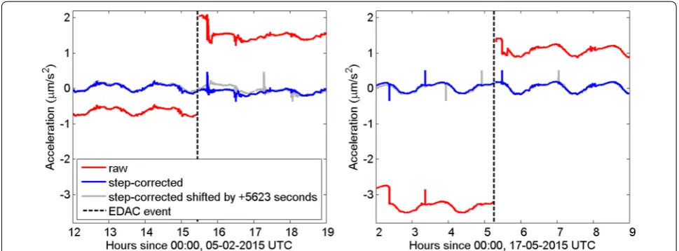
During the power cycling of the accelerometer, the proof-mass position and attitude is not controlled and therefore the proof mass most likely touches the wall stops and thereby discharges. This results in a large step at the EDAC failure event, which is illustrated in Fig. 4. Clearly, the red curves that show the raw accelerations
experience a large step at the epochs of the EDAC failure events, where the step size is typically in the order of sev-eral µm/s2.
Furthermore, we observe a larger number of steps in the raw accelerations during the first and second orbit after an EDAC failure event. For some EDAC failure events, there is almost no effect visible after step correc-tion, whereas for other EDAC failure events, the first and second orbit after an EDAC failure event seem to be of degraded quality. This is demonstrated in Fig. 4, where the blue curves show the step-corrected acceleration and the gray curves show the step-corrected acceleration shifted by one orbit (5623 s) into the future. By compar-ing the blue and gray curves, we see that the accelerations do not change much from one orbit to the next before the EDAC failure events. After the EDAC failure events, the left panel shows differences in the order of 200 nm/s2 that are most likely an artifact of the EDAC failure event, whereas the right panel of Fig. 4 shows almost no changes from one orbit to the next in step-corrected accelera-tions. Thus, accelerations after EDAC failure events must be interpreted with caution. The reason for the different behavior is not known.
Calibration and correction
We assume in this paper that the accelerations experi-enced by the accelerometer cage have a linear relation-ship to the electrode voltages. Thus, the conversion from electrode voltages to accelerations involves the applica-tion of a scale factor and an bias, for which nominal val-ues are known from the design of the accelerometers. It is expected that the real scale factor and bias differ from the nominal ones. Because the control voltages applied to the electrodes are too small for lifting the proof mass in a 1-g environment (Fedosov and Pereštý 2011), the real scale factor and bias cannot be determined on-ground. Instead, they have to be determined in-flight when the accelerometers are in a micro-g environment.
Fig. 3 Representative example of a thruster spike in raw along-track accelerations of Swarm C on July 4, 2014. The thruster spike is due to the activation of the attitude thrusters during nominal satellite operations
Table 1 List of EDAC failure events on the Swarm C accel-erometer in the period from June 2014 to May 2015
Date Time (UTC)
September 4, 2014 17:23:07
September 8, 2014 17:16:57
October 12, 2014 01:35:48
January 29, 2015 13:23:41
February 5, 2015 15:26:44
March 9, 2015 02:32:30
May 17, 2015 05:15:30
May 23, 2015 19:17:18
In practice, we use the nominal scale factor and bias to calculate “raw accelerations.” In order to compensate for the deviation of the real scale factor and bias from the nominal ones, we determine a scale factor and bias for the raw accelerations. We refer to the latter scale factor and bias as calibration parameters. In addition, we con-sider that the bias is not constant, but the slowly drifting difference between the mean value of the raw measure-ments and that of the true accelerations.
For previous missions, a time series of these calibra-tion parameters was estimated by using the accelerom-eter data to represent the non-gravitational accelerations in an orbit determination process using the GPS data as tracking observations, over daily arcs (Helleputte et al. 2009). Unfortunately, the approach described above can not be directly applied to the Swarm mission because biases and scale factors cannot be estimated without correcting also for the above-described disturbances. At least the temperature correction would need to be esti-mated together with the biases and scale factors. How-ever, the temperature correction includes a nonlinear parameter as described in more detail in “Temperature correction” section, which would make the approach unreasonably complicated. Instead, we adopt the prin-ciple of divide and conquer by separating the estimation of non-gravitational accelerations from GPS data and the calibration of the accelerometer data. As a reference to calibrate against, we therefore use accelerations that are estimated from the GPS tracking data, independently from the accelerometer measurements, in a Precise Orbit Determination (POD) process (van den IJssel and Visser 2007).
On Swarm, the accelerometer proof mass is not exactly located in the satellite center of mass. The difference is
in the order of a few centimeters, mainly in along-track direction. The calculation of the location of the satellite center of mass takes into account the amount of fuel left in the tanks and is based on the on-ground characteriza-tion of the satellites in balance tests and measurements of the satellite geometry. The latter included also the determination of the location of the accelerometer proof mass.
The accelerometer will therefore be sensitive to accel-erations due to the gravity gradient between the center of the accelerometer proof mass and the satellite center of mass, as well as to the centrifugal accelerations due to the satellite rotation, which we need to account for. Since the reference accelerations obtained from GPS tracking do not contain the influence of these accelerations, we have to remove them beforehand.
The model for calibration reads
where t is the epoch, acal(t) are calibrated accelerations representing non-gravitational accelerations, s(t) is the scale factor, araw(n) are measured accelerations, bs(t) is the step correction, agg(t) is the acceleration due to the gravity gradient, aca(t) is the centrifugal acceleration, bT(t) is the temperature-dependent part of the bias, and b(t) is the temperature-unrelated part of the bias. It should be noted that Eq. (1) does not model changes of the scale factors due to steps or temperature variations. The reason is that we expect such scale factors changes to be smaller than 1 %, which we consider to be negligible in view of the magnitude of the other disturbances. In the following sections, we describe how s(t), bT(t), and b(t) are estimated.
(1) acal(t)=s(t)∗(araw(t)+bs(t))−agg(t)
−aca(t)+bT(t)+b(t)
Step correction
The correction model for steps foresees to apply a differ-ent bias after the epoch of a step. The model for the step correction bs(n) in Eq. (1) is thus indeed a step function. Since our efforts to correct for steps in an automated way provided unsatisfying results so far, we corrected steps in along-track accelerations of Swarm C manually for the period from June 1, 2014, to May 31, 2015, using a dedi-cated software tool. Most steps do not follow a step func-tion exactly, but show an unpredictable transifunc-tion from one bias level to the next as illustrated in Fig. 1. For this reason, we flagged the accelerations 20 s before and after each of the step epochs and replaced the flagged accelera-tions by linearly interpolated acceleraaccelera-tions using the first good accelerations outside of that time window.
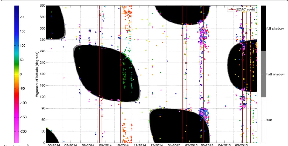
In total, 1510 steps were corrected. Figure 5 shows that steps occur more likely during specific periods, in par-ticular the second half of October 2014 and the first half of March 2015. This is noteworthy as also the GPS receiv-ers on-board Swarm A and C, which fly in a close forma-tion, experienced a number of tracking losses, most likely due to ionospheric scintillations. Moreover, steps are more likely to occur at eclipse transitions, shortly before entering and after leaving the eclipse. It is also worth-while noting that steps often occur in pairs, in the sense that a step of a certain size is followed by another step of almost the same size in the opposite direction, and that
such pairs of steps occur in groups. This means that the accelerometer bias switches back and forth between two distinct levels during some periods.
The result of the step correction is illustrated in Fig. 6. Clearly, the measured accelerations (red curve) show an erratic behavior, neither resembling the accelerations from POD (black curve) nor the temperature inside the accelerometer (gray curve), whereas the step-corrected accelerations (blue curve) show a compelling correlation to temperature. Figure 6 demonstrates that the step cor-rection as well as temperature corcor-rection is very impor-tant parts of the processing.
Temperature correction
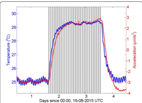
The measured accelerations are correlated with tem-perature to a level where the temtem-perature-induced accelerations exceed by far the real non-gravitational accelerations, which we could already see in Fig. 6. In order to investigate the relation between accelerations and temperature closer, in Fig. 7 we show step-corrected along-track accelerations and the temperature measured by the first temperature sensor inside the accelerometer on Swarm C. The measurements were taken during a thermal test for exploring the capabilities of the heaters to reduce the temperature variations at the orbital period.
Prior to the thermal test, which started at 15:46 UTC on August 17, 2015, both heaters were inactive,
so that the uncontrolled temperature variations could be observed. During the test, both heaters were active approximately 50 % of the time during one orbit, increas-ing the temperature inside the accelerometer by 4 ◦C. After the test, which ended at 13:46 UTC on August 19, 2015, the heaters were inactive again. We can clearly see in Fig. 7 that the accelerations are highly correlated with temperature.
Another important observation in Fig. 7 is that the accelerations increase later than temperature at the beginning of the test and also drop later than tempera-ture at the end of the test. The accelerations show thus a delayed response to temperature changes that we need to take into account when modeling the temperature sensitivity. For this reason, we developed a temperature
correction that models the heat transfer from the tem-perature sensor (point A) to the location where the accel-erometers are sensitive to temperature (point B).
The derivation of the temperature correction begins with the linearization of the temperature at location B.
The temperature change dTB
dt is equal to the heat transfer rate PA→B per heat capacity CB (Lienhard IV and Lien-hard V 2008, p. 8)
For PA→B>0, heat is transferred from location A to location B, whereas for PA→B<0 heat is transferred in the opposite direction. Heat transfer could be caused by conduction or radiation. Judging from experience with thermal vacuum tests during the development of the accelerometers, radiation heat transfer is the more likely candidate for causing temperature changes in a space environment. It can be modeled by
where kA,B is a parameter depending on physical con-stants, surface areas, sensitivities, and geometry (Lien-hard IV and Lien(Lien-hard V 2008, p. 32). Substituting Eq. (4) in Eq. (2) yields
which is the basic model for radiation heat transfer between two locations. In principle, this equation can be the basis for building a complex model for heat trans-fer between many diftrans-ferent locations. We would need to
(2) TB(t+�t)=TB(t)+�t
dTB
dt t
,
(3) dTB
dt = PA→B
CB
(4) PA→B=
TA4−TB4kA,B
(5) TB(t+�t)=TB(t)+�t
TA(t)4−TB(t)4 kA,B
CB , Fig. 6 Result of step correction of along-track accelerations of Swarm C in the period from June 1, 2014, to May 31, 2015
establish a system of equations, where each line would be an equation like Eq. (5). Thus, in theory we could take all available temperature sensors into account for mod-eling the heat transfer to a number of locations inside the accelerometer. However, we prefer the simplest model that is able to correct for the temperature sensitivity. We found through extensive testing
to be a suitable temperature correction, where TA(t) is
the temperature measured by the first temperature sen-sor inside the accelerometer and TB(t) is calculated according to Eq. (5). This choice is motivated by the fact that the first temperature sensor is closest to the solar panels, which gives the largest heat input, compared to the other temperature sensors inside the accelerometers.
Validity periods
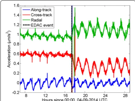
The characteristics of the accelerations change some-times abruptly, which is illustrated in Fig. 8. For the cross-track and radial accelerations, we clearly see that the amplitude at the orbital period changes by a factor of approximately three after the EDAC event. We believe that this is mainly caused by a significant change of the temperature-dependent bias because a change of the scale factor by a factor of three is very unlikely accord-ing to the discussion in “Steps” section. Nevertheless, it seems reasonable to assume that also the other calibra-tion parameters, including the scale factor, change due to the EDAC event. This shows that the calibration and tem-perature correction parameters are only valid for specific
(6) bT(t)=bATA(t)+bBTB(t)
periods. Though the changes in characteristics are much smaller for the along-track accelerations compared to the cross-track and nadir accelerations, it is reasonable to assume that also the parameters for the along-track accelerations have to be exchanged at the epoch of the abrupt change.
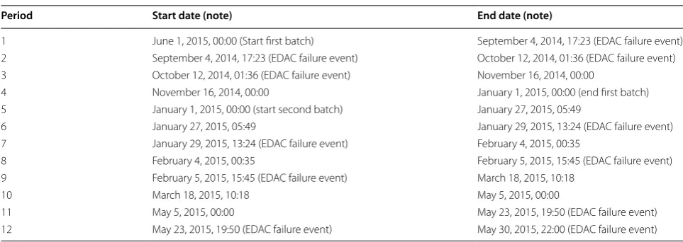
We spent a considerable effort to identify the valid-ity periods for the calibration and temperature correc-tion parameters, which was performed largely by visual inspection. In the end, we identified the 12 validity peri-ods listed in Table 2. Six of the abrupt changes can be associated with a power cycling of the accelerometer due to the occurrence of an EDAC failure event, whereas one change of parameters at the end of year 2014 is simply attributed to the fact that the processing was performed in two batches. The remaining five abrupt changes were found by visual inspection and could not be linked to any particular event.
Non‑gravitational acceleration from precise orbit determination
The non-gravitational accelerations derived through precise orbit determination play an essential role in the processing since they provide the reference signal for the calibration of the accelerometer data. Whereas the scale factors can also be estimated only from accelerometer data collected during a dedicated satellite maneuver as described later in “Scale factor calibration maneuver” section, the estimation of the biases and the tempera-ture correction rely on the non-gravitational accelera-tions derived through precise orbit determination. We describe in this section the processing that is used to determine the latter.
The high-quality GPS receivers on board the Swarm satellites provide near-continuous observations with excellent geometric information due to the low Earth orbits, which allows a precise orbit determination with an accuracy of a few cm. The orbits are the result of all gravitational and non-gravitational forces acting on the satellites. Since models of the Earth’s gravity field have improved significantly due to the dedicated gravity mis-sions CHAMP, GRACE, and GOCE, an accurate extrac-tion of the non-gravitaextrac-tional acceleraextrac-tions from GPS satellite-to-satellite tracking observations is possible (van den IJssel and Visser 2005), albeit at much smaller reso-lution along the orbit than accelerometers provide. On the upside, the non-gravitational accelerations are much more accurate than accelerometers at long periods.
The employed data processing for deriving non-grav-itational accelerations is based on precise orbit deter-mination. The orbit computations are performed with the GEODYN software, which uses a standard Bayes-ian weighted batch least-squares estimator (Pavlis et al. Fig. 8 Identification of validity periods for calibration and
2006). The precise kinematic orbits for Swarm are pro-vided by the SCARF consortium and have an accuracy of about 4–5 cm as validated by independent satellite laser ranging (van den IJssel et al. 2015a). Close to the geo-magnetic poles and along the geogeo-magnetic equator the kinematic orbits show larger errors due to ionospheric scintillations. However, van den IJssel et al. (2015b) show that the optimized receiver settings that were recently uplinked to the Swarm GPS receivers significantly reduce these errors.
Instead of directly using the GPS tracking observa-tions for the determination of non-gravitational accelera-tions, kinematic orbits are used as pseudo-observations. That approach has already been successfully used by, e.g., Visser and van den IJssel (2016) to estimate calibra-tion parameters for the individual accelerometers of the GOCE satellite. Highly reduced-dynamic orbits are fitted to the kinematic orbits, where the gravitational accelera-tions are prescribed by state-of-the-art models (e.g., for the mean gravity field and tides) and the non-gravita-tional accelerations are coestimated. The latter are repre-sented by 3D piecewise linear functions that have 10-min time resolution and are expressed in the same satellite body-fixed frame that is used also for the accelerometer measurements.
To avoid a possible degraded quality of the recovered non-gravitational accelerations at the edges of the orbit arc, and to facilitate overlap analysis, the orbits are pro-cessed in 30 h batches, with 6 h overlaps between sub-sequent orbits. Only the non-gravitational accelerations that are estimated for the central 24 h part of the orbit arc are used for the processing of the accelerometer meas-urements and thermospheric neutral densities.
Using proper constraints for the empirical accelerations can significantly improve the accuracy of the estimated
non-gravitational accelerations (van den IJssel and Visser 2005). For the Swarm satellites, a constraint of 150 nm/s2 is used for the x axis, which is approximately in along-track direction. For the y axis (≈ cross-track direction) a constraint of 80 nm/s2 is used and 50 nm/s2 is used for the z axis (≈ radial direction). These initial values are based on the expected order of magnitude of the non-gravitational accelerations. The constraints can be further optimized using, e.g., overlap analysis. This independent optimization method does not require prior knowledge of the estimated non-gravitational signal and can be used to find near-optimal constraints when gravity field model errors are small (van den IJssel and Visser 2005).
Generally, the accuracy of the estimated non-gravi-tational accelerations is highest for the x axis (≈ along-track direction) due to the strong effect of accelerations in flight direction on orbital dynamics. Predominantly, the longer wavelengths are well determined and high-frequency accelerations, e.g., caused by geomagnetic storms, are less well recovered (van den IJssel and Visser 2007).
Scale factor calibration maneuver
The step-corrected accelerations are highly correlated with temperature, which is demonstrated in Fig. 6. Con-sequently, it is difficult to estimate the scale factor s reli-ably together with the temperature sensitivities bA and bB in a fit against non-gravitational accelerations from POD. For this reason, we designed a special satellite maneuver for the scale factor calibration.
During the maneuver the thrusters are repeatedly activated for 10 seconds, which creates a sequence of large, sharp signals that serve as reference accelerations. The latter are calculated by dividing the nominal thrust force by the satellite mass. We expect that the reference Table 2 Validity periods
Period Start date (note) End date (note)
1 June 1, 2015, 00:00 (Start first batch) September 4, 2014, 17:23 (EDAC failure event) 2 September 4, 2014, 17:23 (EDAC failure event) October 12, 2014, 01:36 (EDAC failure event) 3 October 12, 2014, 01:36 (EDAC failure event) November 16, 2014, 00:00
4 November 16, 2014, 00:00 January 1, 2015, 00:00 (end first batch) 5 January 1, 2015, 00:00 (start second batch) January 27, 2015, 05:49
6 January 27, 2015, 05:49 January 29, 2015, 13:24 (EDAC failure event) 7 January 29, 2015, 13:24 (EDAC failure event) February 4, 2015, 00:35
8 February 4, 2015, 00:35 February 5, 2015, 15:45 (EDAC failure event) 9 February 5, 2015, 15:45 (EDAC failure event) March 18, 2015, 10:18
10 March 18, 2015, 10:18 May 5, 2015, 00:00
11 May 5, 2015, 00:00 May 23, 2015, 19:50 (EDAC failure event)
accelerations have an error of 5–10 % due to small devia-tions of the real thrust force and direction from the nom-inal ones and uncertainties in the satellite mass due to the calculation of the remaining fuel from pressure sensors. We note that the thrusters activations described here should not be confused with those in “Thruster spikes” section since the first are intended to create a linear force in opposition to the latter.
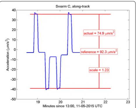
We calculated the scale factor by the ratio of the peak-to-peak reference accelerations and the peak-peak-to-peak measured accelerations. Figure 9 shows the results from the calibration maneuver on May 11, 2015, for the along-track accelerometer axis, where the peak-to-peak refer-ence acceleration was 92.3 µm/s2 and the peak-to-peak measured acceleration was 74.9 µm/s2, which yields a scale factor of 92.3/74.9=1.23.
We notice in Fig. 9 that the bias after each thruster acti-vation is not the same as before. We observed this effect not only for the presented calibration maneuver, but for all calibration maneuvers performed so far. We can see the bias changes most clearly after the second and forth thruster activation at 13:19:20 UTC and 13:20:20 UTC, respectively. We note that these thruster activations were preceded by thruster activations in the opposite direction and that the proof mass moves by approximately 1 µm in response to the thruster activations. We suspect that the position, to which the proof mass returns after the thruster activation, depends on the position of the proof-mass movement during the thruster activation. Since the peak accelerations are typically well repeated, we believe that the bias is affected by hysteresis, though the reason for this is not understood.
It should be noted that we do not use the orbit con-trol thrusters because the resulting acceleration would be outside of the measurement range of the accelerom-eter. Instead, we use special combinations of attitude thrusters that create a linear acceleration that is inside the measurement range. The sequence of thruster activa-tions is designed such that the maneuver has practically no impact on the satellite orbit and attitude. The dura-tion of the thruster activadura-tions is selected to be as short as possible to create a distinct signal that is still within the accelerometer measurement bandwidth, where the upper limit is 0.1 Hz. As a side effect, the fuel consump-tion due to the maneuver is minimized. More details on the maneuvers for scale factor calibration can be found in Siemes et al. (2015).
Estimation procedure
The parameters of the model for calibration and correc-tion of step-corrected acceleracorrec-tions are estimated by a least-squares fit against non-gravitational accelerations from POD, i.e., we minimize the norm ||apod−acal||. The
only nonlinear parameter is the heat transfer parameter kA,B/CB, for which we use a simple line-search to find the best-fitting estimate.
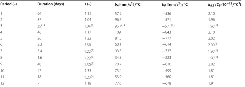
The estimated parameter values are listed in Table 3. For some of the validity periods, it was not possible to estimate the scale factor s or the heat transfer parameter kA,B/CB or both. The reasons are that the validity period was either too short or contained too many steps for a reliable estimation. In those cases, we prescribed the parameter value based on our best knowledge and expe-rience from the other periods. For one period, we used the scale factor determined by the calibration maneuver illustrated in Fig. 9.
The bias that is estimated at this processing stage serves the purpose of absorbing otherwise not modeled effects like the drifting accelerometer bias, accumulated errors from the step correction, and residuals temperature effects. We use quadratic b-splines as basis functions for the bias b where the node distance is typically between 1 and 3 days. We would like to emphasize that the bias of this processing stage shall be considered as an arbitrary parameter that is needed to obtain good estimates for the other parameters. Nevertheless, the bias b is provided in the ACCCCAL_2_ products along with the other terms in Eq. (1).
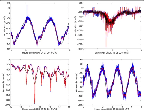
The calibrated and corrected accelerations of Swarm C are compared to accelerations from POD in Fig. 10. The top left panel shows the result of the calibration and correction for 04:00–08:00 UTC on July 4, 2014, as a typical example for Swarm C. There is a good agreement between the calibrated and corrected accelerations (blue
line) and the those from POD (black line), in particular for the phase and the amplitude at the orbital period. We can also see that the accelerometer measures signals at periods much shorter than the orbital period, which are not captured by the accelerations from POD. We also note a spike at 05:07 UTC in the calibrated and corrected accelerations, which is not due to a thruster activation. Since such spikes occur occasionally, we applied a mov-ing-median with a window length of 31 seconds to the calibrated and corrected accelerations (red line) in order to removes spikes and lower the noise level.
In the top right panel of Fig. 10, we show the compari-son for March 16–19, 2015, which is the time when the St. Patrick’s day geomagnetic storm occurred. We high-light the very good agreement between the calibrated and corrected accelerations and the accelerations from POD for the large-scale signal structure, where the accel-erations drop from −200 to −700 nm/s2 during half a day and then increase again to −200 nm/s2 during a bit more than one day. For the finer signal structures, we see differ-ences up to 800 nm/s2 between calibrated and corrected accelerations and the accelerations from POD. This is shown in more detail in the bottom left panel of Fig. 10, which zooms in on 12:00–18:00 UTC on March 17, 2015, where we can see that the difference are due to short and strong negative accelerations that are not well captured in the accelerations from POD due to their 10-min time resolution.
The bottom right panel of Fig. 10 shows the compari-son for 00:00–06:00 UTC on June 25, 2014. In this exam-ple, the accelerations from POD are positive during a small part of the orbit. Since the calibrated and corrected accelerations are fitted against the accelerations from POD, they show the same feature, which is physically
not meaningful since positive accelerations correspond to negative thermospheric neutral densities. The feature occurs predominantly in the period from June to August 2014 when the mean drag is low. It should be noted that the processing of accelerations from POD is not yet opti-mized for Swarm, which implies that we expect improve-ments in the future.
Frequency slicing
In the previous section, we used the non-gravitational acceleration from POD for estimating the calibration parameters. In this section, we go one step further and describe how we fully exploit the synergy between accel-erations and non-gravitational accelaccel-erations from POD. The first are accurate at higher frequencies, whereas the latter are accurate at lower frequencies. Therefore, a com-bination method that we call frequency slicing was devel-oped for merging both types of accelerations. It should be noted that we do not apply the bias b in Eq. (1) because it served as an arbitrary parameter.
Both types of accelerations are differently sampled. Since the signal-to-noise ratio of the calibrated accel-erations is poor at higher frequencies, we decimate those to a sampling rate of 0.1 Hz after applying a 31-s moving-median filter for antialiasing and outlier rejec-tion. The non-gravitational accelerations from POD are linearly interpolated to the epochs of the decimated accelerations.
The resulting acceleration time series are then subdi-vided into overlapping segments, where each segment covers 30 days and the overlap is 11 days. This idea is inspired by Welch’s method for estimating a PSD (Welch 1967). For each segment, we transform the acceleration time series into the frequency domain using a discrete Table 3 Estimated calibration and temperature correction parameters
Values marked by superscript (1) were prescribed based on best knowledge and experience. The value marked by superscript (2) resulted from a calibration maneuver Period (–) Duration (days) s (–) bA [(nm/s2)/◦C] bB [(nm/s2)/◦C kA,B/CB (10−12/◦C3)
1 96 1.11 57.9 −536 2.10
2 37 1.04 96.7 −571 1.96
3 35(1) 1.04(1) 96.7(1) −571(1) 1.96(1)
4 46 1.17 109 −843 2.10
5 26 1.22 81.5 −777 2.02
6 2.3 1.08 60.1 −614 2.00(1)
7 5.4 1.22(1) 93.5 −737 1.90(1)
8 1.6 1.22(1) 34.3 −223 1.90(1)
9 40 1.30(1) 70.7
−616 2.02
10 47 1.33 73.4 −599 1.81
11 18 1.23(2) 53.9
−560 1.81
Fourier transform. Next, we form the weighted aver-age at each frequency, where the weights depend on the frequency. The weights for the non-gravitational accelerations from POD are larger than the weights for the calibrated accelerations below 0.1 mHz and smaller above. Then, we transform the weighted average to the time domain using an inverse discrete Fourier transform. Finally, we reconstruct the merged accelerations from the overlapping segments, using a linear transition from one segment to the next within the overlap.
The result of the method is illustrated in Fig. 11, which shows the PSD of the non-gravitational accelerations from POD, calibrated accelerations without bias applied, and merged accelerations. Since the frequency band in which the weights change smoothly from one to zero is very narrow, the method is somewhat similar to applying
a low-pass filter to non-gravitational accelerations from POD and a complementary high-pass filter to calibrated accelerometer accelerations. This can be clearly seen in Fig. 11, where the PSD of the merged accelerations is practically identical to the PSD of the calibrated accel-eration above 0.1 mHz and non-gravitational accelera-tions from POD below 0.1 mHz. The large peaks above 0.1 mHz reflect the signal at the orbital frequency and its harmonics. We can see that the non-gravitational accel-erations from POD provide only signal up the second orbital harmonic.
isolated from the measurements, by subtracting modeled radiation pressure accelerations.
Here, aae represents the aerodynamic acceleration derived from the measurements, while asrp, aalb, and air represent the contributions to the radiation pres-sure from the Sun, from the Earth’s albedo and from the Earth’s infrared radiation, respectively. These values are available in the ACCC_AE_2_ data product, which will be useful for scientists who might want to study the derivation of densities from accelerations using their own aerodynamic modeling.
The computation of the radiation pressure accelera-tions, making use of a panel model of the satellite outer surfaces, a conical solar eclipse model, as well as maps of the Earth’s albedo reflectivity and IR emissivity, is described in Doornbos (2011). The Swarm-specific panel model properties that have been applied were obtained from ESA and are provided in Table 4.
The conversion of the aerodynamic acceleration meas-urements aae(t) to thermospheric neutral densities ρ(t) is explained in detail by Doornbos et al. (2010), who com-pare so-called direct and iterative methods. The iterative method, introduced in that paper, involves the simultane-ous estimation of crosswind and density, leading to lower errors, but it requires that well-calibrated accelerations from two accelerometer axes are available. Since for Swarm C, we have focused our efforts on the x axis (flight direc-tion) acceleration data only, this method is not available to us, and we will revert to the more simple direct method. Using this method, the density ρ can be related to the aero-dynamic acceleration in the X-direction aae,x as follows:
(7) aae(t)=acal(t)−asrp(t)−aalb(t)−air(t)
The components of this equation will be shortly discussed in turn below.
The spacecraft mass m is provided in the Level 1b sat-ellite data. It is computed from information on the pre-launch dry mass, propellant mass, and used propellant, computed from the temperature and pressure readings in the spacecraft telemetry. During the period of investiga-tion, this mass was about 434 kg, and it changed by less than 1 kg, because no significant orbit or attitude maneu-vers were performed.
The relative velocity of the atmosphere with respect to the spacecraft Vr is calculated according to Doornbos
et al. (2010), by adding the following three components: (1) inertial spacecraft velocity obtained from the GPS-derived orbit (≈7600 m/s, predominantly along-track); (2) the velocity of the corotating atmosphere at the sat-ellite altitude and latitude (up to 500 m/s at the equator, cross-track, zero at the poles); and (3) an estimate of the wind velocity obtained from the HWM07 model (Drob et al. 2008) (up to a few hundreds of m/s, both along-track and cross-along-track).
The aerodynamic force coefficient Cae is obtained using Sentman’s equations (Sentman 1961; Sutton 2009) for a flat panel, by summing the aerodynamic force contri-butions of each of the Swarm surface panels in Table 4 and normalizing by using some reference area Aref. This
same reference area should be used again in Eq. (8) to denormalize the acceleration. Therefore, the reference area value does not matter, and we just used 1 m2. Note
(8) ρ= 2m
ArefV2 r
aae,x
Cae,x
Fig. 11 PSD of non-gravitational accelerations from POD, calibrated accelerations without bias applied, and merged accelerations of Swarm C for the period June 2014 to May 2015
Table 4 Properties of the Swarm panel model used for aer-odynamic and radiation pressure modeling
Panel Area X Y Z
Nadir 1 1.540 0.0 0.0 1.0
Nadir 2 1.400 −0.19766 0.0 0.98027 Nadir 3 1.600 −0.13808 0.0 0.99042 Solar array +Y 3.450 0.0 0.58779 −0.80902 Solar array −Y 3.450 0.0 −0.58779 −0.80902
Zenith 0.500 0.0 0.0 −1.0
Front 0.560 1.0 0.0 0.0
Side wall +Y 0.753 0.0 1.0 0.0 Side wall −Y 0.753 0.0 −1.0 0.0 Shear panel nadir front 0.800 1.0 0.0 0.0 Shear panel nadir back 0.800 −1.0 0.0 0.0
Boom +Y 0.600 0.0 1.0 0.0
Boom −Y 0.600 0.0 −1.0 0.0
that the subscript x for aae,x and Cae,x in (8) indicates that we are only using the X-component of these vectors in the spacecraft body-fixed frame. With all other param-eters known, the density ρ can then be solved from this equation.
Thermospheric neutral densities
The density data, which are the output of all the above processing steps, are available in the DNSCWND_2_ data product. Despite the name of this product, at this point it does not include any wind data. The determina-tion of crosswind data from Swarm accelerometer data is not possible until a stronger drag signal is achieved (at lower altitudes and higher solar activity levels). In addi-tion, this would require a full correction and calibration of the y axis accelerations.
The resulting density data are plotted in Fig. 12, as a function of time on the x axis and the argument of lati-tude on the y axis. The argument of latitude is the angle along the orbit, measured from the ascending node, so that 0◦
and 180◦
correspond to the ascending and descending equator crossings, respectively, while 90◦ and 270◦
correspond to the northern- and southernmost points in the orbit. The variation of solar and planetary geomagnetic activity is indicated in the bottom panels, through the use of the F10.7 and ap proxies.
The left panel of Fig. 12 shows the variation of density over the entire period that was processed so far. It is clear that this period started with very low densities in June and July 2014, due to the high orbit and low solar activ-ity conditions at the time. Much higher densities were reached in December 2014, when solar and geomag-netic activity were higher. The orientation of the orbital
plane of the satellite was such that the daytime density bulge was sampled during descending passes, which cor-responds with the maximum densities being reached between 180◦
and 270◦
argument of latitude during December 2014. In fact, the broad X-shaped pattern in the left panel is due to the slow precession of the orbital plane with respect to the Sun, modulated slightly by sea-sonal density variations and more prominently by varia-tions of solar activity.
The right panel of Fig. 12 zooms in on 10 days sur-rounding the largest geomagnetic storm during the observation period, which happened on March 17 and 18, 2015. This is the so-called St. Patrick’s day storm. The figure clearly shows the more than three times increase in density during the storm, with respect to the quiet conditions prior to the storm. It is also clear to see that the increase in density, caused mainly by increased Joule heating due to ionospheric currents in the auroral zones, started and peaked at high latitudes (around 90◦
and 270◦ argument of latitude). The hotter and therefore denser gas subsequently propagated toward lower latitudes over the course of the next orbits.
A more detailed investigation of this storm or the den-sity data in general is beyond the scope of this paper; however, Fig. 12 clearly demonstrates that such investi-gations, which were previously performed using CHAMP and GRACE data, are now possible using Swarm C data.
Summary and outlook
We presented the processing required for transform-ing the raw accelerations, which are affected by a large number of disturbances, into scientifically valu-able thermospheric neutral densities. Though it provided
Fig. 12 Swarm C densities as a function of time and argument of latitude (upper panels) and solar and geomagnetic activity indices F10.7 and ap
satisfying results, the developed processing scheme should be considered as a pathfinder, for which we see room for improvement in each processing stage:
• The tool for manual correction of the steps could be improved such that it performs a semi-automatic step correction. In view of processing data from Swarm A and B, there might be the need to extend the tool to also handle other disturbances than steps.
• The temperature correction model currently takes the temperature from one sensor inside the accel-erometer as input for modeling the heat transfer to one additional location. As we gain experience, the temperature correction model is expected to become more complex.
• The procedure for estimating the calibration and cor-rection parameters is basic and could be improved, e.g., by incorporating covariance matrices of the observations.
• The method for merging the calibrated accelera-tions with non-gravitational acceleraaccelera-tions from POD was inspired by Welch’s method (Welch 1967). The potential of other methods like the one developed by Stummer et al. (2011) still needs to be investigated.
• The non-gravitational accelerations from POD are not yet optimized for Swarm. Improvements in their determination will facilitate the calibration of the step-corrected accelerations and directly improve the merged accelerations.
We selected data of Swarm C as input for the processing since it seems to be the least affected by the instrumen-tal disturbances. We expect to encounter new challenges when processing data from Swarm A and B, which could necessitate further additions to the processing scheme. With time, the altitude of the Swarm satellites will decrease, thereby increasing the non-gravitational accel-eration signal. The expected higher signal-to-noise ratio should enable us to further improve the quality of the resulting density data.
Despite the large effort invested in improving the pro-cessing, the presented data set is still affected by a num-ber of limitations. The most serious limitation is caused by the temperature sensitivity of the accelerations, where we can split the discussion into three frequency ranges: the sub-orbital frequency range, the orbital frequency and its first harmonic, and the frequency range above the first harmonic of the orbital frequency.
The raw accelerations are clearly dominated by the temperature-dependent bias in the sub-orbital fre-quency range. This is mitigated by the temperature cor-rection described in “Temperature correction” section
to a large extend and any residual temperature effects are then removed using the frequency slicing described “Frequency slicing” section. We believe therefore that the quality of aerodynamic accelerations and thermospheric neutral densities is good for sub-orbital and longer periods.
The phase and amplitude of the orbital signal in the raw accelerations is heavily perturbed by the tempera-ture-dependent bias. We fully rely on the quality of the accelerations from POD for finding a good temperature correction. However, the orbital signal and its first har-monic are at the limit of the time resolution that the accelerations from POD provide. This leads sometimes to unwanted effects like the positive accelerations shown in Fig. 10 and discussed in “Estimation procedure” sec-tion. We expect that an optimization of the processing of accelerations from POD for Swarm will improve the situation.
On the positive side, the temperature variations show no signal in the frequency range above the first harmonic of the orbital frequency. This means that we expect no negative impact of the temperature sensitivity in that frequency range. Here, the quality of calibrated and cor-rected accelerations is dominated by the quality of the scale factor and the number of short-lived disturbances like spikes. Due to the calibration maneuvers, we expect that the scale factor is known to 5–10 % as discussed in “Scale factor calibration maneuver” section. The num-ber of spikes in Swarm C along-track accelerations is fortunately not high. We observe on average less than one spike per orbit in the period from June 2014 to May 2015 and we note that spikes can be mitigated by apply-ing a movapply-ing-median to the calibrated and corrected accelerations.
The processing of Swarm accelerometer data has proven to be much more challenging than the processing of accelerometer data from other missions like CHAMP, GRACE, and GOCE. We expect that the experience and knowledge gained from Swarm data can to some extent be transferred to the other missions, as they might be subject to some of the same effects, though in a much more subtle way.
The investigations have focused so far on the linear acceleration measurements. The accelerometer also measures the angular accelerations, which could be used to improve the satellite attitude product. This will be sub-ject to future investigations.
Authors’ contributions
The presented paper is the result of a team effort as indicated in the following. CS contributed to analysis of the disturbances, evaluated the temperature sensitivity using the data collected during dedicated heater tests, performed part of the step correction and the calibration against accelerations from POD, performed the temperature correction, developed the scale factor calibration maneuvers, and coordinated the team effort. JE contributed to analysis of disturbances and developed and performed the frequency slicing. ED contrib-uted to analysis of the disturbances and temperature sensitivity, performed part of the step correction, the conversion to aerodynamic accelerations and thermospheric densities. JIJ calculated the accelerations from POD. JK contributed to analysis of the disturbances, evaluated the temperature sensi-tivity, developed the temperature correction model, and provided technical expertise on the instrument. RP contributed to analysis of the disturbances, evaluated the temperature sensitivity, and provided technical expertise on the instrument. LG contributed to analysis of the disturbances and supported the development of the scale factor calibration maneuver. GA and JF contributed to the analysis of the disturbances. PEHO contributed to analysis of the distur-bances and supported the coordination of the team effort. All authors read and approved the final manuscript.
Author details
1 RHEA for ESA - European Space Agency, Noordwijk, Netherlands. 2 Delft
University of Technology, Delft, Netherlands. 3 Serenum, a.s., Prague, Czech
Republic. 4 Helmholtz-Zentrum Potsdam, Deutsches GeoForschungsZentrum,
Potsdam, Germany. 5 Leibniz Universität Hannover, Hannover, Germany. 6 DTU
Space, Technical University of Denmark, Kongens Lyngby, Denmark.
Acknowledgements
The European Space Agency is acknowledged for providing the data. The GEODYN software was kindly provided by the NASA Goddard Space Flight Center. We would like to thank Aleš Bezděk and Sean Bruinsma for their thor-ough analysis of two test data sets and valuable feedback on the data quality.
Received: 31 December 2015 Accepted: 18 May 2016
References
Bruinsma S, Tamagnan D, Biancale R (2004) Atmospheric densities derived from CHAMP/STAR accelerometer observations. Planet Space Sci 52(4):297–312
Chvojka M (2011) Microaccelerometer error analysis. In: Chzech aerospace proceedings, number 1. www.vzlu.cz/download.php?file=510
Doornbos E (2011) Thermospheric density and wind determination from satel-lite dynamics. PhD thesis, Delft University of Technology
Doornbos E, Den IJssel JV, Lühr H, Förster M, Koppenwallner G (2010) Neutral density and crosswind determination from arbitrarily oriented multiaxis accelerometers on satellites. J Spacecr Rockets 47(4):580–589
Drob DP, Emmert JT, Crowley G, Picone JM, Shepherd GG, Skinner W, Hays P, Niciejewski RJ, Larsen M, She CY, Meriwether JW, Hernandez G, Jarvis MJ, Sipler DP, Tepley CA, O’Brien MS, Bowman JR, Wu Q, Murayama Y, Kawamura S, Reid IM, Vincent RA (2008) An empirical model of the Earth’s horizontal wind fields: HWM07. J Geophys Res 113:A12304. doi:10.1029/ 2008JA013668
Fedosov V, Pereštý R (2011) Measurement of microaccelerations on board of the LEO spacecraft. In Preprints of the 18th IFAC World Congress. http:// www.nt.ntnu.no/users/skoge/prost/proceedings/ifac11-proceedings/ data/html/papers/1873.pdf. Milano (Italy) Aug 28–Sept 2
Helleputte TV, Doornbos E, Visser P (2009) CHAMP and GRACE accelerom-eter calibration by GPS-based orbit daccelerom-etermination. Adv Space Res 43(12):1890–1896
Lienhard JH IV, Lienhard VJH (2008) A heat transfer textbook, 3rd edn. Phlogis-ton Press, Cambridge
Pavlis DE, Poulouse SG, McCarthy JJ (2006) GEODYN operations manuals contractor report. SGT Inc., Greenbelt
Sentman LH (1961) Free molecule flow theory and its application to the determination of aerodynamic forces. Tech Rep LMSC-448514. Lockheed Missiles & Space Company
Siemes C, Doornbos E, de Teixeira da Encarnação Ja, Grunwaldt L, Pereštý R, Kraus J (2015) Calibration of Swarm accelerometer scale factors. Tech Rep SWAM-GSEG-EOPG-TN-15-0008, Issue 1, Revision 0, ESA—European Space Agency
Stummer C, Fecher T, Pail R (2011) Alternative method for angular rate deter-mination within the GOCE gradiometer processing. J Geod 85:585–596 Sutton EK (2009) Normalized force coefficients for satellites with elongated
shapes. J Spacecr Rockets 46(1):112–116
Sutton EK, Nerem RS, Forbes JM (2007) Density and winds in the thermo-sphere deduced from accelerometer data. J Spacecr Rockets 44(6):1210– 1219. doi:10.2514/1.28641
van den IJssel J, Visser P (2005) Determination of non-gravitational accelera-tions from GPS satellite-to-satellite tracking of CHAMP. Adv Space Res 36(3):418–423
van den IJssel J, Visser P (2007) Performance of GPS-based accelerometry: CHAMP and GRACE. Adv Space Res 39(10):1597–1603
van den IJssel J, Encarnação J, Doornbos E, Visser P (2015a) Precise sci-ence orbits for the Swarm satellite constellation. Adv Space Res 56(6):1042–1055
van den IJssel J, Forte JB, Montenbruck O (2015b) Impact of Swarm GPS receiver updates on POD performance. submitted to EPS. Earth Planets Space 68:85. doi:10.1186/s40623-016-0459-4
Visser P, van den IJssel J (2016) Calibration and validation of individual GOCE accelerometers by precise orbit determination. J Geod 90(1):1–13. doi:10.1007/s00190-015-0850-0
Welch PD (1967) The use of Fast Fourier Transform for the estimation of power spectra: a method based on time averaging over short modified peri-odograms. IEEE Trans Audio Electroacoust 15(2):70–73