Modeling, Analysis and Control of Oscillations in Wind-integrated Power Systems.

ABSTRACT

CHANDRA, SOUVIK. Modeling, Analysis and Control of Oscillations in Wind-integrated Power Systems. (Under the direction of Aranya Chakrabortty.)

In this dissertation work, we assess the impacts of high wind penetration on the operational aspects of conventional power system and propose methods for planning and control to ensure a secure operation. Analytical models of the wind-integrated power system are derived where wind turbine is connected to the power grid asynchronously via doubly fed induction generators (DFIG). Particularly we focus on the equilibrium and the electromechanical oscillation spectrum of the power system. Our study illustrates that the wind power locations affect the oscillation spectrum particularly the inter-area or slow oscillation of the power system. We design damping controllers on the wind generator and associated storage to minimize the undesired influence of wind on the oscillations enabling an efficient operation of the power system. Further analysis shows that the wind power alters the equilibrium characteristics in a power system and give rise to slow and poorly damped inter-area oscillatory modes under certain scenarios, by significantly affecting the bus voltages of the power system. We also propose a numerical homotopy based method which is capable of identifying multiple equilibrium and the power flow solution boundary of the wind-integrated power system.

First, in Chapter 2, we analytically show the impact of wind power injection on the spectral response of a large radial power system, represented as a continuum model. The inter-area oscillation spectrum of the power system is found to be significantly affected by the location of the wind injection in the power system. Accordingly in Chapter 3, we design a linear controller for the wind generator to shape inter-area oscillation spectrum in a desired pattern. Particularly it is shown that the performance of the wind farm controller in shaping the inter-area oscillation spectrum can be considerably improved by a coordinated control action with a battery energy system (BES).

derived consisting of synchronous generators, wind turbines interfaced with a DFIG, loads and transmission lines. Considering a power system with multiple coherent areas of operation, we analytically show how the slow or inter-area oscillatory modes get affected by increasing wind penetration. Simulation studies suggest that depending on the relative locations of the synchronous generators, the wind generator and the loads, there might be scenarios in which the inter-area oscillatory mode gets slower with higher wind injection ultimately leading to instability.

©Copyright 2015 by Souvik Chandra

Modeling, Analysis and Control of Oscillations in Wind-integrated Power Systems

by Souvik Chandra

A dissertation submitted to the Graduate Faculty of North Carolina State University

in partial fulfillment of the requirements for the Degree of

Doctor of Philosophy

Electrical and Computer Engineering

Raleigh, North Carolina 2015

APPROVED BY:

Iqbal Husain Mo-Yuen Chow

Fen Wu Aranya Chakrabortty

DEDICATION

BIOGRAPHY

ACKNOWLEDGEMENTS

I would like to thank my advisor, Dr Aranya Chakrabortty , for his extensive help throughout the duration of my PhD research career here at NC State. Without his help, technical advice, and mentoring, this wouldn’t have been possible. The experience of working with him has been great, particularly the one-to-one conversations that we have had over the past few years were very productive. I would like to thank him for the immense faith that he has shown in my abilities and for grooming me for my future technical endeavors.

I would also like to thank all the other members in my thesis committee, namely, Professors Iqbal Husain, Mo-Yuen Chow and Fen Wu, for carefully reviewing my work and providing me with valuable feedback to improve my work. I am indebted to my collaborators Dr Dennice Gayme from Johns Hopkins University and Dr Dhagash Mehta from University of Notre Dame who have always been very generous to review my work and helping me with ideas. Also I would like to extend my sincere thanks to all the other Professors in the the FREEDM Systems Center for giving me an exposure to state-of-art research topics and training environment. Not only the Professors, I should thank all the staff as well, especially Mrs Keren Autry, for their immense help in administrative matters and making my life easy.

and deeply encouraged my academic endeavors. On a whole I was blessed with great teachers throughout my academic career who helped me to keep ablaze my constant zeal to learn and reinvent myself.

My graduate life at Raleigh would have been much dull if I had not met all those wonderful friends both in my neighborhood and in the FREEDM lab. I shared my stay here with my roommate Prithwish Bhaumik who has been a great companion and supported me in my every endeavor. I enjoyed the company of many of my neighbors in our Raleigh Community like Ayan Dasgupta, Sayantan Banerjee, Rudrodip Majumdar, Rajarshi Dasbhowmik, Priyam Das, Raj Bhakta, Shuva Gupta, Lopamudra Kundu and many others. I appreciated the company of my lab mates as well during my duration at the FREEDM systems center with whom I had constant interactions on technical issues and shared a strong bonding of friendship. I would like to mention Sayan Acharya, Ritwik Chattopadhyay, Samir Hazra, Ankan De, Sachin Madhoosodan, Awneesh Tripathi, Ali Safayet, Govind Chavan, Byron Beddingfield, Behzad Nabavi, Thomas Nudell, Almuatazbellah Boker, Urvir Singh, Sumit Dutta, Tanvir Khan, Nan Xue, Abhishek Jain, Matthew Weiss, Jianhua Zhang, Faeza Hafiz and many others.

TABLE OF CONTENTS

List of Tables . . . .viii

List of Figures . . . ix

Chapter 1 Introduction . . . 1

1.1 Background . . . 1

1.1.1 Types of Wind Integration Technologies . . . 2

1.1.2 Small Disturbance Rotor Angle Stability Dynamics . . . 4

1.1.3 Transient Voltage Stability . . . 6

1.2 Contributions . . . 7

1.3 Organization . . . 7

Chapter 2 Spectral Response of a Wind-injected Power System Model . . . 9

2.1 Continuum Representation of a Radial Power System with a Point Wind Injection 10 2.2 Wind Farm Model . . . 13

2.3 Computation of the Spectral Response of the Wind-injected Power System . . . 14

2.4 Simulation Results . . . 15

2.4.1 Spectral Response of the Wind Farm . . . 16

2.4.2 Spectral response of the Power Flow in the Grid . . . 16

2.5 Conclusions . . . 17

Chapter 3 Damping of Inter-area Oscillations in Power Systems: A Frequency Domain Approach . . . 19

3.1 Centralized Control Design for Spectral Matching . . . 20

3.1.1 Wind Farm Model and Controller Design . . . 20

3.1.2 BES Model and Controller Design . . . 24

3.1.3 Spectral Analysis . . . 27

3.1.4 Simulation Results . . . 30

3.2 Disaggregation of Control from Equivalent Turbine to Multiple Turbines . . . . 31

3.2.1 Centralized Design . . . 32

3.2.2 Decentralized Design . . . 33

3.2.3 Simulation Results . . . 34

3.3 Conclusions . . . 37

Chapter 4 Time Scale Modeling of Power Systems with Wind Injections . . . 38

4.1 Wind Integration Modeling . . . 40

4.1.1 Synchronous Generator Model . . . 40

4.1.2 Wind Power Plant Model . . . 42

4.1.3 Wind Integrated Power System Model . . . 46

4.2 Time-scale Modeling . . . 48

4.2.1 Power System Time-constants . . . 49

4.2.3 The Effect of Wind Injection on Time-scales . . . 53

4.3 Results . . . 55

4.3.1 2-area 8-bus Power System . . . 56

4.3.2 5-area 68-bus Power System . . . 58

4.4 Conclusions . . . 61

Chapter 5 Equilibria Analysis in Wind-integrated Power Systems . . . 63

5.1 Dynamic Model of Power System . . . 64

5.1.1 Synchronous Generator Model . . . 64

5.1.2 WPP Model . . . 66

5.1.3 Dynamic Load Model . . . 70

5.1.4 Power Flow Model . . . 70

5.2 Equilibrium Analysis . . . 71

5.3 Parameter Homotopy Continuation Algorithm . . . 73

5.4 Results . . . 76

5.4.1 Discussion: On the Network Topology and Upper Bound on the Number of Equilibria . . . 78

5.5 Background for Power Flow Solution Boundary . . . 79

5.6 Examples . . . 82

5.6.1 3-bus System . . . 82

5.6.2 10-bus system . . . 85

5.7 Conclusions . . . 86

Chapter 6 Conclusions and Future Works . . . 88

References. . . 91

Appendix . . . 98

Appendix A Simulation Parameters . . . 99

A.1 Model Parameters for Two-area Kundur System . . . 99

A.2 Wind Plant Parameters . . . 99

LIST OF TABLES

Table 2.1 List of principle symbols in Continuum model of the Power System . . . . 11 Table 3.1 List of principle symbols in BES model . . . 26 Table 3.2 Optimal controller parameters sets . . . 30 Table 3.3 Optimal controller parameters sets . . . 36 Table 4.1 Matrix norms and slow eigenvalues for the 8-bus 4-machine 2-area power

system. . . 57 Table 4.2 Fast eigenvalues for the 8-bus 4-machine 2-area power system in different

scenarios. . . 58 Table 4.3 Matrix norms and slow eigenvalues for the 68-bus 16-machine 5-area power

system. . . 59 Table 5.1 Types of feasible equilibrium for various wind speeds (v_re) and wind bus

voltage levels|Ve

w6| . . . 76

LIST OF FIGURES

Figure 2.1 A radial power system of generators subject to wind injection at a distance

α along the transfer path. . . 12

Figure 2.2 Frequency and time domain response of the power output from the lin-earized wind farm model in (2.23) . . . 17

Figure 2.3 Spectral response of power flow of a wind-integrated power system for different wind farm power injection locations α. . . 18

Figure 3.1 Steady-state speed versus power characteristics of a 1 MW wind turbine. The maximum power curve, shown in red, depicts the operating points for each wind speed. . . 21

Figure 3.2 Two-loop control scheme for wind turbine in which the inner loop controls generator speed set points shown in Figure 3.1 while the outer loop is the proposed power controller for shaping the inter-area oscillation spectrum of the grid. . . 22

Figure 3.3 Battery Energy System (BES). . . 23

Figure 3.4 Spectral response comparison . . . 31

Figure 3.5 Schematic for the disaggregated wind farm control, where each turbine is controlled individually, and the total power output of the farm is aggregated and injected to the grid at the point of common coupling. . . . 32

Figure 3.6 Comparison of spectral matching between the aggregate versus disaggre-gated wind farm model . . . 34

Figure 3.7 Arrangement of turbines in the wind farm. . . 36

Figure 3.8 Open-loop versus closed-loop δ(t) at u= 0.25 with slow mode components 37 Figure 4.1 Wind turbine interfaced to the grid via a DFIG . . . 41

Figure 4.2 Decoupled active and reactive power control of a DFIG integrating a wind generator via the rotor-side controller . . . 43

Figure 4.3 Kundur 8-bus, 4-machine, 2-area power system with wind injection at bus 5 55 Figure 4.4 Kundur 8-bus, 4-machine, 2-area power system with wind injection at bus 7 56 Figure 4.5 68-bus, 16-machine, 5-area power system: Scenarios with wind injection at bus 66 and at bus 38 . . . 62

Figure 5.1 Dynamic model of a Wind integrated power system . . . 65

Figure 5.2 Schematic representation of the WPP and the power system . . . 66

Figure 5.3 3-bus power system with two parameters . . . 81

Figure 5.4 Power flow solution boundary tracking with various initial points . . . 83

Figure 5.5 10-bus power system with 2 WPP . . . 84

Chapter 1

Introduction

1.1

Background

This has lead to an enormous amount of research on various topics related to power system planning and operations with high wind penetration, which includes reliability analysis [75], security [78], wind-centric electricity markets [69], and demand response [9]. A significant amount of work has also been carried out on component-level modeling and control of wind turbines with relevant power electronic interfaces [21, 79, 98]. A few works have focused on operational concerns of the power system as well, such as frequency regulation and load following [19, 38] or mitigating the risks associated with variability and uncertainty in wind power production using operating reserves [51], storage [8] or demand-side management [90]. However, only a modest amount of research has been directed towards gaining a theoretical understanding of how wind power generation affects the dynamic behavior of power systems that are dispersed over large geographical areas. The majority of the work on this topic has focused on component-level analysis of the impacts of integrating doubly-fed induction generators (DFIG) in the grid [83, 91] using simulation-based case studies [25, 70, 95] that doesn’t provide much theoretical insights. Also a general framework for analysis and control of system-level dynamic power system model in presence of substantial wind penetration is missing. Thus the primary focus of this dissertation work is to derive theoretical models for wind-integrated power system in order to investigate the impact of penetration levels on the dynamic power system model, particularly on equilibrium and small disturbance rotor-angle oscillation dynamics. As a background review, we discuss the various wind integration technologies, the concepts of small disturbance rotor angle dynamics, equilibria analysis and transient voltage stability of power system.

1.1.1 Types of Wind Integration Technologies

uses a blade and hub rotor assembly to obtain wind power and transfer it to a generator at a higher speed through a geared shaft. Since the wind speed varies, the generator speed also needs to vary for which the most popular form of wind integration is through asynchronously means via induction generators. Primarily the classification of the wind turbines is based on the speed of the generator, fixed speed (type-I) or variable speed type (type II-IV) and the related technologies [79, 89]. The details of these technologies for the wind turbines are given as below

Type I These wind turbines are of fixed-speed type and are used primarily in small utility-scale applications. They have a fixed turbine rotor speed even even the wind speed varies. They are thus interfaced with squirrel-cage induction machines, with the stator directly connected to the grid and the rotor short-circuited. Even though the technology is fairly robust, cheap and simple, lack of efficiency and inability to compensate reactive power to the grid are some of its major disadvantages.

Type II These wind turbines are of variable-speed type which can operate at a given range of rotor speeds as the wind speed changes to ensure efficiency. These turbines often are provided with blade and pitch control which improves efficiency as compared to fixed speed types. Here the variable speed of the machine is maintained via the dynamic rotor resistance control where the resistance in the rotor circuit of the machine is allowed to change for a certain range of operating slip speeds.

reactive power capability of the generator. In our work we focus on this type of wind generators and will derive the detailed dynamic model of this type of wind generators in 3.

Type IV These wind turbines use full converters where the wind turbine is connected only via the back-to-back AC/DC/AC converter to the grid. These turbines may employ synchronous generators, induction generators or permanent magnet machines which offer full independent real and reactive power control.

Next we review the rotor angle dynamics of conventional power systems.

1.1.2 Small Disturbance Rotor Angle Stability Dynamics

in the dynamic response of the phase angles and frequencies. The fast time-scale arises from the relative motions of the local generators inside an area, which synchronize quickly due to their strong interconnections reaching a so called quasi-steady state. The states from the different areas, thereafter, synchronize with each other over a slower time-scale, giving rise to inter-area oscillations. A constructive analysis of this behavior is also common in the literature. For example, to obtain an analytical expression for the fast and slow oscillation dynamics, one may define the slow or aggregate variable for thekth _{area to be the so-called center of inertia angle} for that area, namely

yk,

Pnk

i=1Mikδik

Pnk

i=1Mik

, k= 1,2, ...r (1.1)

where δ_ik and M_ik are, respectively, the ith machine angle and inertia in thekth area,nk is the total number of machines in thekth area, and r is the total number of areas. Similarly, the fast variable for thekth area can be defined as

zk,i,δki −δ1k, i= 1,2, ...nk, k= 1,2, ...r. (1.2)

The time-scale separation between the fast and slow oscillations can then be expressed explicitly in the singular perturbed form

dy dts

= A11y+A12z,

dz dts

=A21y+A22z (1.3)

where 1 is a small parameter, and the exact expressions for the four state matrices can be found in [18]. Assuming≈0, the effective swing dynamics for the inter-area oscillations can then be written as:

dy dts

= (A11−A12A−221A21)y. (1.4)

It must be noted that the matrix (A11−A12A−221A21) is not necessarily block-diagonal, and

levels of wind penetration on these oscillations have also been the subject of a number of recent studies [26, 91, 95] which shows some results based on simulation case studies. But in this work we look to theoretically capture the effect of wind penetration on the oscillatory modes from the analytical model of the wind-integrated power system. We also validate the findings from the theoretical model with relevant case studies using standard IEEE models.

1.1.3 Transient Voltage Stability

Voltage stability is related to the ability of the power system to maintain voltages at all of its buses to some steady value following a disturbance at a given initial condition [44]. Small-signal or transient voltage stability is related to maintenance of steady voltages under small disturbance [24, 44]. Wind penetration has a significant impact on the equilibrium characteristics of a power system which is closely related to small-signal transient voltage stability. It has been well established in literature that wind generators interfaced with doubly-fed induction generators can be particularly beneficial during short term voltage instability owing to their reactive power capability as compared to older fixed speed induction generators [81, 97]. However how the amount of penetration and location of the wind injection affects the equilibrium characteristics is missing in literature. We tried to address this issue by showing how in a multiple wind-injection scenario the power system equilibrium is parameterized by the wind variables. Thereafter we use a parameter homotopy based computational method to identify all the equilibria of the power system. Next we use the same procedure to identify the relative penetration levels in a multiple-wind scenario where the power flow solution boundary occurs, the knowledge of which is crucial to maintain voltage security from a planning perspective. The traditional methods for solving these problems [35] depends upon initial guess and local approximations. However the proposed method is independent of initial guess and guarantees to find all solution boundaries in a given parameter space.

1.2

Contributions

1. Coordinated controller design for wind farms and battery energy systems for inter-area oscillation damping in power systems via spectral matching.

2. Derivation of the wind-integrated power system model where wind turbines are interfaced to the grid via a DFIG.

3. Time-scale modeling of wind-integrated power systems and analysis of the effect of increasing wind penetration on the inter-area modes.

4. Equilibria analysis of wind-integrated power systems via numerical homotopy method and determination power flow boundary or transient voltage stability limit.

1.3

Organization

In Chapter 2, of this thesis, we derive an approximate continuum model of a large radial power system network with wind injection at a point location. We show analytically that the spectral response of this system is a function of the location of the wind injection. Particularly our simulation results based on a two-area power system model inspired by the Pacific AC Inter-tie demonstrate that the inter-area oscillation spectrum of the power system is highly dependent on the location of wind injection.

locations of the wind farm and the BES, and can be implemented in a decentralized fashion. In Chapter 4, we derive a pertinent mathematical model for the wind-integrated power system consisting of synchronous generators, loads and a wind plant driven by a DFIG. We aggregate this system into multiple coherent areas, and apply a linear transformation to represent the model in terms of slow and fast states. Using this transformed system we show that the ratio of the time constant associated with the swing states to that of the wind plant can be used to characterize conditions under which the slow time-scale of the power system changes with increasing wind penetration. We further demonstrate that these modal responses depend on the relative locations of the synchronous generators, the loads and the wind generator through simulation examples in a two-area 8-bus power system and a five-area 68-bus power system.

Chapter 2

Spectral Response of a

Wind-injected Power System Model

Inter-tie.

2.1

Continuum Representation of a Radial Power System with

a Point Wind Injection

Consider a string of ngenerators distributed along a normalized spatial dimension u∈[0,1]. At each bus i, we define the set ˜Ei := {Ei, δi}, where δi is the rotor phase angle and Ei is the voltage magnitude in figure 2.1. The line reactance and distance between generators iand

i+ 1 are respectively denoted xi and ∆L. The dynamics of the ith generator is given by the electro-mechanical swing equation as shown below,

2Hi Ωs

¨

δi+ζδ˙i =Pi ∀i= 1,2...n (2.1)

where Ωs= 120π= 377 rad/s is the electrical frequency (assuming a 60 Hz base), Pi is the net active power flowing out of theith machine (P0 = 0) andζ is the damping coefficient. The real

power flow from nodeitoi+ 1 over a purely reactive line is given by,

Pi,i+1=

EiEi+1sin(δi−δi+1)

xi

. (2.2)

We simplify (2.2) by considering a linear power flow approximation and constant voltages. Thus, we assume small angle differences (i.e. the sine function can be approximated by a linear difference) and constant voltage, which without loss of generality means we can set Ei = 1 (p.u.). The expression for net active power flowing out of theith machine then becomes

Pi=Pi−1,i−Pi,i+1=

1

xi−1

(δi−1−δi)− 1

xi

(δi−δi+1). (2.3)

δi Rotor angle of theith generator in figure 2.1

Hi Inertia of theith generator in figure 2.1

ξi Damping of theith generator in figure 2.1

Ei Internal voltage of theith generator in in figure 2.1

Pi Power output of theith generator in figure 2.1

Pi,i+1 Power flow from theith to the (i+ 1)th generator in figure 2.1

δ(u, t) Aggregate rotor angle at locationu and timetin (2.4)

ν Propagation velocity of the wave equation (2.4)

γI Impedance density of the wave equation (2.4)

Pg(t) Wind farm power output

Table 2.1: List of principle symbols in Continuum model of the Power System

following damped hyperbolic wave equation in terms of the aggregate generator angle δ(u, t)

∂2δ(u, t)

∂t2 +ξ

∂δ(u, t)

∂t =ν

2∂2δ(u, t)

∂u2 . (2.4)

The wave speed is defined as

ν =

r

377 2HTγI

. (2.5)

In (2.4) and (2.5),ξ,HT, andγIrespectively denote the damping, inertia, and reactance densities over the string of generators, which are derived in [20, 27]. In the continuum these densities take the form

HT = 1

L

Z L

0

dH(u) = H(L)

L , γI = x(L)

L , η= ζ(L)

L . (2.6)

For ndiscrete generators one can approximate H(L) =Pn

i=1Hi,x(L) =Pni=1xi, andζ(L) =

Pn

i=1ζi. The corresponding continuum expression for the power flow associated with (2.4) is

P(u, t) =−1 γI

∂δ(u, t)

∂u . (2.7)

Generator Converter

( )

g

T t Zg( )t

Drive Train Aerodynamics

( )

ref t

E

( )

r t

Q

( )

a

T t

( )

r t

Z

P

jx

jx

P

P

P

1

~

E

E

~

E

~

E

~

1

H

H

3

H

H

u

0 L

L

ȴ

D

_{(1- )}

_D

Figure 2.1: A radial power system of generators subject to wind injection at a distanceαalong the transfer path.

(2.4) can be written as

∂2δ ∂t2 +ξ

∂δ ∂t−ν

2∂2δ

∂u2 =Pg(t)ˆδ(u−α) (2.8)

where ˆδ(u−α) is the dirac-delta function, used to represent a spatial point source at u=α. We assume that the power flow at the boundaries are constant over time implying that

δ(u, t) is a standing wave with zero slope at the boundaries [20]. The change in the power at the two ends of this tie-line can be used to define the following boundary conditions for (2.8),

∂δ ∂u

u=0

=

∂δ ∂u

u=1

= 0. (2.9)

2.2

Wind Farm Model

In this section we derive an aggregate model for a wind farm based on a single equivalent

wind turbine. Later we will generalize this assumption to include multiple wind turbines whose individual power outputs are added at a point of common coupling, and injected to the grid. We consider the nonlinear wind turbine model consisting of a two-mass drive train, induction generator and aerodynamic torque as presented in [92]. The drive train is modeled as two connected shafts operating at high and low speeds with respective inertiasJrandJg, and friction coefficientsBr and Bg. The transmission gear connecting the shafts has a gear ratio of Ng, and a torsion stiffness and damping of Kdt and Bdt, respectively. The model is represented in state space in terms of its 4 states namely turbine rotor speed ωr(t), the generator torsion angleθ(t), generator speedωg(t) and torqueTg(t) as,

Jrω˙r(t) =

Bdt

Ng

ωg(t)−Kdtθ(t)−(Bdt+Br)ωr(t) +Ta(t) (2.10a)

Jgω˙g(t) =

Bdt

Ng

ωr(t) +

Kdt

Ng

θ(t)−

Bdt

N2

g +Bg

ωg(t)−Tg(t) (2.10b) ˙

θ(t) =ωr(t)− 1

Ng

ωg(t) (2.10c)

˙

Tg(t) =− 1

τg

Tg(t) + 1

τg

Tg,ref(t). (2.10d)

where, Ta(t) is the aerodynamic torque, and Tg,ref is a reference generator torque. The aerody-namic torque Ta(t) is

Ta(t) =

ρAsvr3(t)Cp(t) 2ωr(t)

(2.11)

where ρ is air density, As is the total swept area of the turbine blade, Cp(t) is the power coefficient, andv(t) is the wind speed. The dynamics of (2.10d) are orders of magnitude faster than (2.10a)-(2.10c). We, therefore, assume Tg(t) to be a constant that we denote Tg,ref. The output power generation of the open-loop turbine model is given by

where ηg is the generator efficiency. Pg(t) defines the forcing term in (2.8). We linearize the model (2.10)-(2.11) about an operating point (ωg,0,ωr,0 ,θ0, Tg) and obtain a frequency response for the linearized power flow. The frequency response of the linearized power output of the wind farm is used to compute the frequency response of the power system described in (2.8)-(2.9).

2.3

Computation of the Spectral Response of the Wind-injected

Power System

We next derive an expression for the spectral response of (2.8) in terms of the the wind farm transfer function associated withPg(t). We begin by expressing δ(u, t) andW(u, t) in terms of Fourier series expansion as shown below [27],

δ(u, t) =1 2A0+

∞ X

n=1

[An(t) cos(knu) +Bn(t) sin(knu)] (2.13a)

W(u, t) =1 2F0+

∞ X

n=1

[Fn(t) cos(knu) +Gn(t) sin(knu)] (2.13b)

whereknis the wave number of each modeλn. We assume that the power flow at the boundaries are constant over time implying thatδ(u, t) is a standing wave with zero slope at the boundaries and power flow given as

p(0, t) =p(1, t) = 0. (2.14)

Using (2.14) it is easy to show that Bn(t) =Gn(t) = 0.Then substituting (2.13a) and (2.13b) into (2.8) yields

d2_A

n(t)

dt2 +η

dAn(t)

dt −ν

2_k2

nAn(t) =Fn(t) (2.15) where the Fourier coefficient Fn(t) follows from

Fn(t) = 2

1

Z

0

where

W(u, t) =Pg(t)ˆδ(u−α). (2.17)

Substituting (2.17) in (2.16) and solving we get

Fn(t) = 2Pg(t) cos(knα). (2.18)

Then the frequency response of An(t) from (2.15) depends on the locationα and is given by

An(α, jω) =

2Mn(ω) [cos(θn) +jsin(θn)]

q

(k2

nν2−ω2)

2

+ (ξω)2

(2.19)

where

Mn(ω) =|Fn(jω, α)|, (2.20)

and θn is the phase of An, which is

θn=∠Fn(jω, α)−tan−1

ξω k2

nν2−ω2

. (2.21)

The net spectral response of the power flow, given by (2.8) at a certain location u is given by,

SP(ω, α) = 1

γ2

I

∞ X

n=1

|An(α, jω)|2sin2(knu) (2.22)

2.4

Simulation Results

2.4.1 Spectral Response of the Wind Farm

We first obtain a linearized model of the wind farm described by (2.10)-(2.11) and (2.12) about an operating point (ωg,0,ωr,0 ,θ0,Tg) and represent the system in terms of a transfer function. The transfer function of the wind farm is calculated based on the parameters of the wind farm, given in [92], shown as: Jr = 55×106 kgm2, Jg = 390 kgm2,Br = 27.8×103 Nm/(rads/s),

Bg = 3.034 Nm/(rads/s), Bdt = 945 kNm/(rads/s),Kdt = 2.7×109 Nm/rad, Ng = 95,τg = 10 ms, As= 10387 m2,ρ= 1.225 kg/m3,Tg,ref = 2500 Nm,ηg = 0.92 and an input Ta(t) = 1.6. With these parameters and assumption of Tg(t) = ˜Tg,ref = 2500 Nm for all timet, the transfer function of the wind farm power output is given as,

Gw(s) =

6.786s+ 1.939e004

s3_{+ 0.294s}2_{+ 816.2s+ 0.7696}. (2.23)

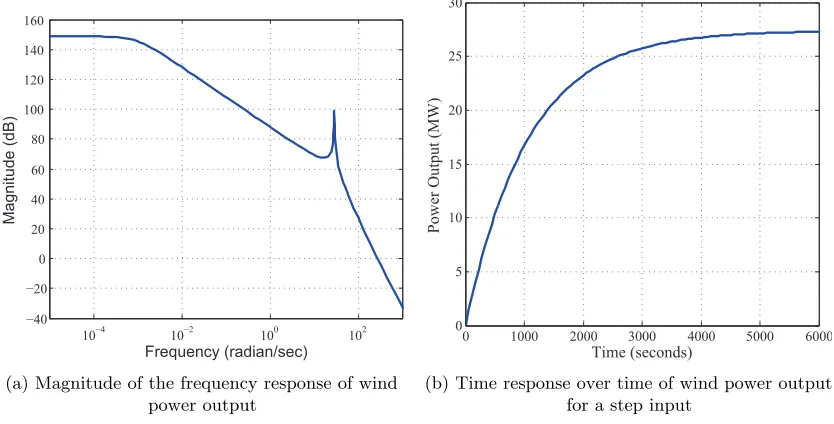
The Bode Magnitude response for the transfer function is shown as Figure 2.2a while Figure 2.2b shows the step response of the transfer function Gw(s) of the wind power output. The spectral response of the wind power output is used to compute the power flow spectrum of the entire power system as shown next.

2.4.2 Spectral response of the Power Flow in the Grid

We compute the spectral response of the power flow in the wind integrated power system derived in (2.22) using the following parametersγI_{= 3.13×10}−3 _{rad/MW,ξ= 0.4 /sec,ν = 0.4 rad/sec}

10−4 10−2 100 102 −40

−20 0 20 40 60 80 100 120 140 160

Frequency (radian/sec)

Ma

g

n

it

u

d

e

(d

B)

(a) Magnitude of the frequency response of wind power output

0 1000 2000 3000 4000 5000 6000 0

5 10 15 20 25 30

Time (seconds)

P

ow

er O

ut

p

ut

(M

W

)

(b) Time response over time of wind power output for a step input

Figure 2.2: Frequency and time domain response of the power output from the linearized wind farm model in (2.23)

or sharp peaks in the spectral response . In the next section we look to desgin the frequency spectrum of the power flow of the grid like a desired response with a wind farm at any arbitrary location using a wind power controller [28].

2.5

Conclusions

0.1 0.2 0.3 0.4 0.5 0.6 0.7 0.8 0.9 1 65

70 75 80 85 90 95 100

Frequency(Hz)

M

ag

n

it

u

d

e(

d

b

)

D=0

D=0.25

D=0.50

D=1.0

Chapter 3

Damping of Inter-area Oscillations

in Power Systems: A Frequency

Domain Approach

In Chapter 2 we have shown results based on a continuum model of a radial power system, which demonstrate that the inter-area oscillation spectrum of the wind-integrated power system is strongly influenced by the wind farm injection locationα [27]. But the location of a wind installation in a geographically diverse power system may be limited by several issues like geographical, economic, political etc. In a situation where the wind farm location is not ideal, it may give rise to poorly damped inter-area oscillatory modes in the power system, detrimental for its normal operation. In this scenario, we aim to design closed loop controllers for the wind farm which can allow us to shape the inter-area oscillation spectrum of the power flow in a desired pattern. We assume that given a frequency range of interest, a particular wind power injection pointα∗ produces the so-called optimal (most desirable) frequency response without any controller. However if the situation is such that a wind farm could not be installed at this

drawback of this approach is that this matching can only be guaranteed over narrow frequency bands necessitating frequent switching of controllers from one band to another.

We provide a means to circumvent this problem by designing co-dependent controllers for the wind farm power output and a controlled Battery Energy System (BES) by which we achieve a better match of the spectral response of the system to the so-called optimal response [11, 14]. Usually many wind installations have a storage associated with it on the same bus to improve their reliability. We look to exploit the available power electronic controllers of the BES for our control design. The design is posed as a parametric optimization problem that minimizes the error between the two spectral functions over a finite range of frequencies. We introduce a realistic two-loop control strategy for the wind speed and power control. This two-loop control system is based on a maximum power-point tracking wind turbine controller, and is, therefore, a more realistic design for real-time implementation [11]. Secondly we develop dis-aggregation methods for implementing controllers at each individual wind turbine instead of using a hypothetical equivalent turbine to represent the wind farm. We illustrate the typical closed-loop dynamic performance trade-offs when aggregate control systems get distributed among individual turbines [11]. Our results take into account the typical power output patterns of the different rows of a wind farm, and, thereby, capture the variations in wind speed due to wake effects.

3.1

Centralized Control Design for Spectral Matching

3.1.1 Wind Farm Model and Controller Design

0 500 1000 1500 2000 2500 3000 3500 0 0.2 0.4 0.6 0.8 1.0 1.2 1.4 1.6 1.8 2.0

ω_g (rpm)

Power (MW)

Increasing wind speed

Maximum power curve

Figure 3.1: Steady-state speed versus power characteristics of a 1 MW wind turbine. The maximum power curve, shown in red, depicts the operating points for each wind speed.

linearized system are then the small-signal changes from the equilibrium that we denote as

ξ= [∆ωg,∆ωr,∆θ]T. We next define the corresponding inputs asφ= [∆vr,∆Tg]T to obtain

˙

ξ =Aξ+Bφ (3.1)

where, A=      

−(Bdt+Br)

Jr −

ρAsv3r,0Cp

2ω2 r,0Jg

Bdt

NgJr −

Kdt

Jr

Bdt

NgJg −

1

Jg(

Bdt

N2 g +Bg)

Kdt

NgJg

1 − 1

Ng 0

      B =      

3ρAsvr,02 Cp

2ωr,0Jg 0

0 −_J1

g 0 0       .

The linearized output equation (2.12) is

+

Ͳ , g ref P

' 'Ta

g T '

6

6

q s q p s p s p

6

LeadͲlag compensator + Ͳ + + g

Z

s r p

r g

A v C

J U

Z 'vr

r

v

'

k

k

k

4

k

k

' g ref,

Z

'

1

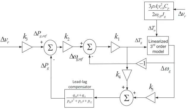
Figure 3.2: Two-loop control scheme for wind turbine in which the inner loop controls generator speed set points shown in Figure 3.1 while the outer loop is the proposed power controller for shaping the inter-area oscillation spectrum of the grid.

Defining the two outputs y= [∆Pg,∆ωg]T, the output equation is given by

y=Cξ+Dφ (3.3)

where C=



 

0 k5 0

0 1 0





, D=



 

0 k4

0 0



 ,

k4:= ηgωg,0 and k5 := ηgTg,ref.

Following standard practice, we assume that the steady-state power output of the turbine is controlled to achieve its maximum power for a given wind speed vr (as shown in Figure 3.1) using a maximum power-point tracking (MPPT) algorithm, e.g. as in [21]. The power output controller that we are going to design in this work will be implemented on top of this MPPT. The control scheme is shown in Figure 3.2, where the constants k1, k2 and k3 are

defined as follows. When the wind speed changes by a small amount ∆vr from the equilibrium speed, the slope k3 of the power versus wind speed characteristics at the point of linearization

Battery Control scheme 3ĭ connection PT CT AC/DC converter

(a) Schematic View

Converter BES P BT R 1 B R 1 B C 1 B V BS R BP

R CBP VBOC

Charging/Discharging circuit Self-Discharging circuit Battery dc u d c i a e b e c e L L L C

(b) Equivalent Circuit Representation

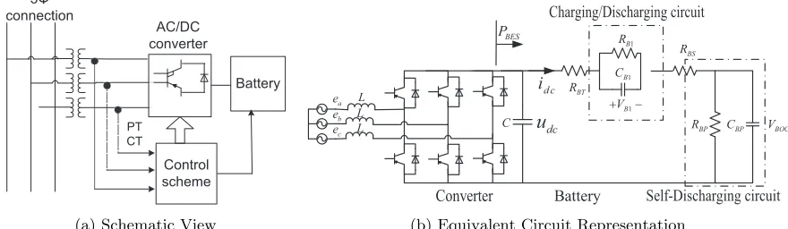
Figure 3.3: Battery Energy System (BES).

power versus generator speed characteristics, in turn, generates a new reference ∆ωg,ref for the generator speed. The product of this speed reference and the slopek1 of the speed versus torque

characteristics is then imparted as the new generator torque, as indicated in Figure 3.1. We first design a unity-gain feedback to regulate ∆ωg to its reference. This loop is referred to as the inner loop, which typically has a bandwidth higher than 10 Hz. The outer loop consists of feeding back both the generator torque and the generator speed, after proper scaling, to control the transient response of the generator output power ∆Pg(t) using a linear feedback controller. In general, there is no restriction on the choice of the outer-loop controller as long as it guarantees closed-loop stability and transient performance. For simplicity, we select a second-order lead-type controller of the form

Gi(s) =

q10s+q11

p10s2+p11s+p12

(3.4)

and define the set of controller parameters S1:={q10, q11, p10, p11, p12}. In the following

3.1.2 BES Model and Controller Design

Here we present the dynamic model of the BES, and derive an expression for its output power

PBES(t), which is going to supplement Pg(t). As shown in Figure 3.3a, the BES model has 4 parts: a three-phase transformer, a pulse-width modulation (PWM) based AC-DC converter, a battery model, and a controller [50]. The transformer is used to step down the grid voltage to the battery level. The battery model usually consists of a set of batteries connected in series or parallel. For our study, however, we will consider an ideal transformer with a single equivalent battery model. The circuit diagram of the BES is given in Figure 3.3b. The necessary circuit analysis and subsequent linearization of the system considered here are described as follows. Table 3.1 provides a list symbols used in the following discussion.

The average model of the three-phase PWM converter shown in Figure 3.3b, assuming a

dq0 reference frame [16], can be expressed as

Ld dt       id iq i0       =       dd dq d0      

udc+

     

0 ω 0

−ω 0 0

0 0 0

            id iq i0       −       ed eq

e0−

√

3un

      (3.5a)

Cdudc

dt =idc−

dd dq d0

      id iq i0       (3.5b)

In this nonlinear converter model the control inputs are the three duty cycles dd, dq and d0.

However, for simplicity, here we limit our control design to only a single-input converter model. For this we consider the small-signal changes of the three duty cycles to be the same, i.e. ∆dd= ∆dq= ∆d0:= ∆d, and use ∆das the effective control input. Note that the equilibrium

input can be written as M1 d dt         

∆id

∆iq

∆i0

∆udc

        

=M2

        

∆id

∆iq

∆i0

∆udc

        

+M3∆d+

         0 0 0 1         

∆idc (3.6)

where,

M1:=diag(L, L, L, C)

M2:=

        

0 ω 0 dd∗

−ω 0 0 dq∗

0 0 0 d0∗

dd∗ dq∗ d0∗ 0         

, M3 :=

        

udc∗

udc∗

udc∗

−(id∗+iq∗+i0∗)

         .

The subscript ‘∗’ denotes the point of linearization. Furthermore, assuming that the converter circuit dynamics is significantly faster than the battery dynamics, or in other words LandC in (3.5a)-(3.5b) are negligibly small, we obtain the following algebraic relationship between the

states [∆id,∆iq,∆i0,∆udc] and the control input ∆d:

        

∆id ∆iq ∆i0

∆udc

        

=−M₂−1M3∆d−M2−1

         0 0 0 1         

∆idc (3.7)

Simplifying (3.7), we obtain

∆udc(t) =

udc∗

d0∗

∆d(t). (3.8)

Analyzing the battery circuit, on the other hand, we get

L andC Filter inductance and dc-link capacitance

ed, eq and e0 dq0 components of the transformer secondary voltage

id, iq and i0 dq0 components of the current at the transformer secondary

dd, dq and d0 dq0 components of the duty cycle

udc andidc Terminal voltage and current of the equivalent battery

ω Synchronous frequency of the grid

un Neutral point voltage

RBT Equivalent resistance of parallel/series connection of batteries

RBS Series resistance of the battery

PBES Active power of the BES

VB1 Battery overvoltage

RB1 and CB1 Charging circuit resistance and capacitance (Figure 3.3b)

RBP andCBP Battery self-discharge resistance and capacity (Figure 3.3b)

Table 3.1: List of principle symbols in BES model

wherer1 := _1+sRR_B1B1_CB1 andr2:= _1+sRR_BPBP_CBP,RBT is the equivalent resistance of a parallel/series connection of batteries, and RBS is the internal resistance of the battery. The parallel circuit of RBP and CBP is used to represent the self discharge of the battery while the charging or discharging circuit corresponds to a parallel combination of RB1 and CB1. The small-signal

expression of the active power fed to the system is then given by

∆PBES =udc0∆idc+idc0∆udc. (3.10)

Substituting (3.8) and (3.9) in (3.10), we obtain a transfer function of the system as

∆PBES(s) =

udc0

F(s) +idc0

udc0

d00

∆d(s) (3.11)

where,

F(s) := RBP +RB1+sRBPRB1(CBP +CB1) (1 +sRBPCBP)(1 +sRB1CB1)

+RBS+RBT.

form

GcBES(s) =

q20s+q21

p20s2+p21s+p22

(3.12)

with parameters S2= {q20, q21, p20, p21, p22}. A unit step response of the closed-loop BES model

is denoted asPBES(t) which is injected in the power system.

3.1.3 Spectral Analysis

A wind farm and a battery energy system (BES) described in subsections 3.1.2 and 3.1.2 repectively, are incorporated in the power system into (2.4). We consider the wind farm power injection Pg(t) and the BES as drawing power PBES(t) as a point source forcing at locationα from one end of the transfer path. This leads to the forced wave equation

∂2δ ∂t2 +ξ

∂δ ∂t −ν

2∂2δ

∂u2 =W(u, t), (3.13)

where

W(u, t) = (Pg(t)−PBES(t))ˆδ(u−α) (3.14)

is the net power injected into the system. We use the dirac-delta function ˆδ(u−α) to represent the spatial point source at u = α. In equation (3.14) we use the convention that PBES ≥ 0 represents charging (i.e. the BES is a power sink) andPBES <0 is discharging (i.e. the PES is a power source). We next derive the expressions for the spectral response of (3.13) in terms of the the closed-loop transfer functions associated with ∆Pg(t) and ∆PBES(t) by applying Fourier series as shown in section 2.3. We begin by expressingδ(u, t) andW(u, t) in terms of Fourier series

δ(u, t) =1 2A0+

∞ X

n=1

[An(t) cos(knu) +Bn(t) sin(knu)] (3.15a)

W(u, t) =1 2F0+

∞ X

n=1

wherekn is the wave number of each mode λn. We assume that the power flow at the two boundaries are zero, i.e.,

p(0, t) =p(1, t) = 0 (3.16)

implying that δ(u, t) is a standing wave with zero slope at the boundaries. Using (2.14) it is easy to show thatBn(t) =Gn(t) = 0.Then substituting (3.15a) and (3.15b) into (3.13) yields

d2An(t)

dt2 +η

dAn(t)

dt +ν

2_k2

nAn(t) =Fn(t) (3.17)

where the Fourier coefficient Fn(t) follows from (3.14) as

Fn(t) = 2(Pg(t)−PBES(t)) cos(knα). (3.18)

The frequency response of (3.18) can be written as

Fn(jw,S1,S2, α) =2 [Pg(jω,S1)−PBES(jω,S2)] cos(knα). (3.19)

The corresponding power flow equation is given by

p(u, α, t) = 1

γI

∞ X

n=1

knAn(α, t) sin(knu). (3.20)

Taking the Fourier transform of (3.20), we get

P(u, α, ω) = 1

γI

∞ X

n=1

knAn(α, ω) sin(knu), (3.21)

where

An(α, ω) =

|F_n(jω,S₁,S₂, α)|

[(k2

nν2−ω2)2+η2ω2]1/2

with θn=∠Fn(jω,S1,S2, α)−tan−1

ξω k2

nν2−ω2

. The net spectral response of the system (2.8) at a certain locationu with the wind farm and BES atα can finally be written as,

SPcl(u, ω,S1,S2, α) =|P(u, α, ω,S1,S2)|

2_{. (3.22)}

From now onwards, we will dropu from the arguments ofSPCL(·) for brevity, knowing that the

frequency response is always computed at a fixed spatial location.

The control problem formulated is to design the parameter sets S₁ and S₂ such that

SPcl(ω,S1,S2, α) at any fixedumatches a desired spectral response over a given frequency range.

In general, this desired spectral response can be chosen arbitrarily depending on the control objective. The formulation of the design pursued in this chapter is as follows. We first consider the open-loop frequency response SP(ω, α) of the wind-integrated power system without the controllersS1 andS2, i.e. (S1 = 0,S2 = 0 in (2.22)). Next, we identify the locationα2 for which

the frequency response over ω∈[ω1, ω2] has the most favorable damping. Ideally, in that case,

one would place a wind farm and BES atα2, but that may not be always possible due to various

geographic, economic and political constraints. Then, one way to solve the problem would be to treat the spectrum atu=α2 as a reference, install the wind farm at a viable locationu=α1,

and design the controllersS1 andS2 such that the spectrumSPcl(ω,S1,S2, α1) closely matches

the reference spectrum over ω ∈ [ω1, ω2]. The controller design can then be written as the

following optimization problem:

min

S1,S2

ω2 Z

ω1

[log(SPcl(ω, α1,S1,S2))−log (SP(ω, α2))]

2_{dω. (3.23)}

Frequency range S1 S2

0.1 to 0.3 Hz [1.604 1.210 0.909 1.392 0.835] [2.354 0.893 1.521 0.059 0.612] 0.3 to 0.5 Hz [1.438 0.785 0.718 1.055 0.313 ] [1.495 1.786 1.844 0.038 1.571] 0.5 to 0.7 Hz [0.836 1.020 0.698 0.917 2.398] [2.455 2.355 0.575 0.976 0.340] 0.7 to 0.9 Hz [1.185 0.951 0.383 0.584 1.317] [0.967 0.192 1.766 1.235 0.808]

Table 3.2: Optimal controller parameters sets

3.1.4 Simulation Results

We consider a case where both the wind farm and the BES are located at α= 0.5, while the system planner desires the controlled spectral response of the grid to match the response of the system corresponding to α∗ = 0.25. Following [50] we assumeβR= 85◦, the transformer secondary voltage as 5 KV,RBT = 0.0167 Ω,RBS = 0.013 Ω,XC0 = 0.0274 Ω,RB1 = 0.001 Ω,

CB1= 1 F,RBP = 10 kΩ, andCBP = 52600 F. We then design controllers of the form (3.4) and (3.12) for the wind farm and BES systems using the procedure described in the subsection 3.1.3.

Figure 3.4 compares the net spectral response this controlled system to the desired response over four different frequency ranges. Figure 3.4a illustrates the results when the optimization algorithm (3.23) is run with ω1 = 0.2π rad/s, ω2= 0.4π rad/s. The corresponding controller

parameters are S₁ = [0 0.067 1.894 1.732 3.276] and S₂ = [0 0.143 1.366 1.176 4.038]. This particular controller does not work well beyond ω2 = 0.4π rad/s. Therefore, we design a new

0.1 0.12 0.14 0.16 0.18 0.2 0.22 0.24 0.26 0.28 55 60 65 70 75 80 Frequency(Hz) Magnitude(db)

windfarm at α*=0.25 controlled windfarm at α=0.5 controlled windfarm and battery at α=0.5

(a) Comparison in the range of 0.1 to 0.3 Hz

0.3 0.32 0.34 0.36 0.38 0.4 0.42 0.44 0.46 0.48 0.5 44 46 48 50 52 54 56 58 60 62 Frequency(Hz) Magnitude(db)

windfarm at α*=0.25 controlled windfarm at α=0.5 controlled windfarm and battery at α=0.5

(b) Comparison in the range of 0.3 to 0.5 Hz

0.5 0.52 0.54 0.56 0.58 0.6 0.62 0.64 0.66 0.68 0.7 54 56 58 60 62 64 66 68 70 72 74 Frequency(Hz) Magnitude(db)

windfarm at α*=0.25 controlled windfarm at α=0.5 controlled windfarm and battery at α=0.5

(c) Comparison in the range of 0.5 to 0.7 Hz

0.7 0.72 0.74 0.76 0.78 0.8 0.82 0.84 0.86 0.88 46 48 50 52 54 56 58 60 62 64 66 Frequency(Hz) Magnitude(db)

windfarm at α*=0.25 controlled windfarm at α=0.5 controlled windfarm and battery at α=0.5

(d) Comparison in the range of 0.7 to 0.9 Hz

Figure 3.4: Spectral response comparison

solving this optimization problem, and generalize theequivalent turbine model to account for a decentralized system with controllers at each individual turbine.

3.2

Disaggregation of Control from Equivalent Turbine to

Mul-tiple Turbines

) ( g

P

) ( 1

g P

) (

2

g

P Pgi( )

) ( gN

P

Turbine # 1 Turbine # 2 Turbine # i Turbine # N

) ( 1 s

C _{( )}

2 s

C Ci(s) CN(s)

1

v v2 vi vN

Figure 3.5: Schematic for the disaggregated wind farm control, where each turbine is controlled individually, and the total power output of the farm is aggregated and injected to the grid at the point of common coupling.

Figure 3.5. This can be done in either of the following two ways.

3.2.1 Centralized Design

Let the total number of turbines in the farm be N. Let the controller for theith turbine be

Gi(s) =

qi0s+q1i

pi0s2+pi1s+pi2

(3.24)

with its parameters denoted by the set S1i ={qi0, qi1, pi0, pi1, pi2}, where i= 1, . . . , N. The

parameters of all N turbines can then be designed in a batch fashion to solve a modified optimization problem

min

S1i,S2

ω2 Z

ω1

[log(SPcl(ω, α,S11, ...,S1N,S2))−log (SP(ω, α

∗_))]2_{dω, i= 1, . . . , N.}

(3.25)

the subsequent rows. For example, the second and subsequent rows typically produce about 60% of the power generated by the first row [87]. The centralized optimization (3.25) searches for the optimal controller parameters to minimize the integral error between the frequency spectra of the wind-integrated power system, and, therefore, will not necessarily guarantee this distribution of row-wise power outputs. Additional constraints may be placed on the search of

S1i and S2 to satisfy this criteria, but that will increase the computational time. To overcome

these shortcomings we next describe an alternative approach.

3.2.2 Decentralized Design

This design consists of two steps. First, solve the optimization problem (3.23) assuming a single aggregate wind turbine with an aggregate controller S1. Then, compute the closed-loop

frequency response Pg(ω) of the total power injected by the wind farm to the grid over the desired frequency rangeω∈[ω1, ω2]. Next, consider that the ith row of the wind farm has Ni turbines, each of them being driven by the same wind speed vr,i. The speed from one row to another will, however, vary because of wake effects. Letpi be the fraction of power expected to be generated by the ith row. The controller design problem can then be stated for each individual turbine as

min

Sj

ω2 Z

ω1

log(Pg,j(ω,Sj))−log

pi

Ni

Pg(ω)

2

dω. (3.26)

where, j refers to a turbine index in the ith row (i= 1, .., N), andPg,j(ωj,Sj) is the closed-loop frequency response of the magnitude of the output power produced by thejth turbine. Since every turbine in theith row tracks the same reference pi

NiPg(ω), (3.26) can be solved for one

0.4 0.45 0.5 0.55 65

70 75 80 85 90 95

Frequency (Hz)

Magnitude(db)

Reference tra jectory(α∗= 0

.25)

Uncontrolled system atα= 0

.5

Controlled distributed system atα= 0

.5

Controlled aggregate system atα= 0

.5

Figure 3.6: Comparison of spectral matching between the aggregate versus disaggregated wind farm model

3.2.3 Simulation Results

Here we illustrate the control designs proposed in subsections 3.2.1 and 3.2.2 for a wind and BES integrated power system using parameters mentioned previously. The power and the energy ratings of the battery are 1 MW and 40 MWh.

Figure 2.3 shows the spectra the wind-integrated power systems with no BES for four different values of α. This figure illustrates that as the wind power injection site is varied from α = 0 to 1 the spectrum shows notable changes in both its period and the frequencies corresponding to the associated peaks and troughs. The variation in frequency response with wind injection location may make the damping at a particular wind injection site more desirable than others. For example, the spectrum for α = 0.5 shows a peak at 0.4 Hz, while that for

α = 0.25 shows a trough that extends over 0.35 to 0.45 Hz. Since our goal is to damp the interarea modes, we select the spectrum associated with α= 0.25 as the reference trajectory (which we denote asα∗), and design a controller for a wind farm located atα= 0.5.

obtained as,

S1 ={0.6075,0.8794,1.2754,1.6246,1.3712} (3.27)

S2 ={0.1207,1.9472,1.6284,1.3772,0.0062} (3.28)

Figure 3.6 shows that the closed-loop frequency response tracks the reference closely in the frequency range of interest. To test the efficiency of our control scheme for other frequency ranges, we also designed the controllers for those ranges assuming an aggregate wind turbine model. The spectral matching for each of these frequency ranges are found to be similar to that shown in Figure 3.6.

Next, we pursue the decentralized control approach described in section 3.2.2, and design individual wind farm controllers using (3.26). We consider a wind farm with 4 rows, each containing 5 turbines, as shown in Figure 3.7. The power production percentages for each row are assumed to be p1 = 36%, p2 = 22%, and p3 = p4 = 21%. Turbines 3, 8, 13, and 18

are chosen as the representatives for their respective rows as they are centrally located, and, therefore, would have the least edge effects. The optimization problem (3.26) is solved for each of these four turbines, and the corresponding parameters for the controllers S₁₁,S₁₂,S₁₃, and S₁₄ are listed in Table 3.3. Every other turbine in the ith row is then controlled using

S1i,i= 1,2,3,4. Figure 3.6 shows that the closed-loop frequency response of the grid power flow resulting from controlling the 20-turbine wind farm and the BES atα= 0.5 matches the reference fairly well over [0.45,0.5] Hz, but has a greater mismatch over [0.4,0.45] Hz. This can be explained by noting that the parameter optimization problem (3.26)) minimizes the integral of the error function over the frequency range [0.4,0.55] rather than a point-to-point matching. For example, as can be seen in Figure 3.6, the undershoot in the range f ∈(0.42,0.45] Hz is partially compensated by the overshoot whenf ∈[0.45,0.52] Hz and f <0.42 Hz. A higher order controller or gain-scheduling may further improve the matching.

To validate our results in the time-domain, we construct δ(u, t) =P16

1 2 3 4 5

6 7 8 9 10

11 12 13 14 15

16 17 18 19 20

1

v

2

v

3

v

3

v

11

S

11

S

11

S

11

S S₁₁

12 S

12

S S₁₂ S₁₂ S₁₂

13

S S₁₃ S₁₃ S₁₃

13

S

13

S

13

S S₁₃ S₁₃ S₁₃

Figure 3.7: Arrangement of turbines in the wind farm.

Row no. Controller Parameters

1 S11 = [ 0.042 0.3016 2.93e4 6566 4.77e6]

2 S16 = [8e-5 0 87.90 53.14 1128.0366]

3, 4 S1,11 = [0.0234 8.6e-3 236.23 3005.76 1.05e5]

Table 3.3: Optimal controller parameters sets

0 5 10 15 20 25 −1

0 1 2

Time (Sec)

δ

(rad)

0 5 10 15 20 25

−1 0 1 2

Time (sec)

δ

(rad)

Uncontrolled phase angle at u=0.25 Slow mode component

Controlled phase angle at u=0.25 Slow mode component

Figure 3.8: Open-loop versus closed-loopδ(t) atu= 0.25 with slow mode components

3.3

Conclusions

Chapter 4

Time Scale Modeling of Power

Systems with Wind Injections

Over the past few decades the operating characteristics of the North American power grid have changed substantially due to increasing penetration of renewable energy resources such as wind. These changes have led to a significant amount of research investigating the challenges associated with large-scale integration of wind energy [8, 9, 51]. The impact of increased levels of wind penetration on grid stability and dynamics [77], and in particular on inter-area oscillations, have also been the subject of a number of recent studies [25, 83, 91, 95]. Methods have been proposed to control these effects by regulating the wind farm power output [11, 79], and by controlling doubly fed induction generators (DFIGs) to increase oscillation damping [70, 95]. However, a detailed, rigorous analytical framework for evaluating the impact of wind penetration on power system oscillations has yet to be developed. Specifically, there is very limited understanding of how wind injection may affect the time-scale separation orcoherency properties of conventional grid models [17].

to each other, and synchronize over a slower time-scale. Using singular perturbation (SP) theory, [17] derived an analytical model describing suchfastandslowmotions for synchronous generators which depend on the relative norms of the network admittance matrices containing external and internal interconnections among generators. The approach in [17,18] was complimented by several related papers such as [29, 84, 99] through various model reduction techniques. Aggregation and coherency are still two of the most fundamental tools that are used to reduce the computational complexity of solving thousands of nonlinear equations in power system stability programs [82], and find wide applications to both small-signal and transient stability assessment [94].

In this Chapter we study how the conventional coherency model of a power system changes due to the addition of wind power. We first derive a mathematical model for the dynamics of a power network consisting of synchronous generators, loads, transmission lines and wind generator. The wind generator is modeled as a group of identical wind turbines electrically connected to the power grid at a point of common coupling via controlled DFIGs. We then aggregate the system into multiple coherent areas, and apply a linear transformation to represent the model in terms of slow and fast states. Using this transformed system we analytically show that the slow oscillatory modes of the power system can be affected by the wind plant depending on the wind penetration level and other power system parameters. Preliminary results on this topic have been recently reported in our conference paper [13]. Here we extend those results to include an explicit model showing the impact of wind penetration on the slow oscillatory modes of the power system [13]. Additionally in this chapter we develop detailed case studies illustrating the conditions when increasing wind penetration alter the slow oscillatory modes of the power system. In particular we explore case studies with different locations of the wind plant in the two-area, four-machine Kundur power system and the five-area, sixteen-machine interconnected power system of the New England (NETS) and New York power systems (NYPS).

provided in section 4.4.

4.1

Wind Integration Modeling

We consider a power system with the set of buses N =: {1, . . . , N} and n generators where

n≤N. These generators consist of a setG=:{1, . . . , n−1} of synchronous generators and one wind power plant. Without loss of generality we can reorder the buses so that theithsynchronous generator is always connected to theith bus and the wind generator is connected to the nth

bus. To understand the coherency properties for this system, we first derive its small-signal electro-mechanical dynamic model considering both swing dynamics of the synchronous machines and the dynamics of the wind power plant.

4.1.1 Synchronous Generator Model

We model the dynamics of each generatori∈ G based on [43] as,

˙

δi =ωi (4.1a)

miω˙i =Pmi−

Ei

x0_di(ViResinδi−ViImcosδi). (4.1b)

Hereδi,ωi,mi,Ei,x0diandPmiare respectively the phase angle, machine speed, inertia, internal machine voltage, direct-axis salient reactance and the mechanical power input to generator

i∈ G, andVi=ViRe+jViIm is the voltage at busi∈ G. Linearizing (4.1) about an operating

point (δ0_i, ω_i0, V_i0 Re, V

0

iIm,P

0

mi) for every i∈ G, the overall small-signal model can be written as

∆ ˙δ=I∆ω (4.2a)

M∆ ˙ω=k11∆δ+k12∆V + ∆Pm (4.2b)

where ∆ indicates a small change of a variable. M is a diagonal matrix of the inertias mi

DC/AC AC/DC

Controller s

i

s

v

r

v

i

Power Grid

( ) g

T t

Drive Train

( ) a

T t

Aerodynamics

( ) r t Q

( )

r

t

Z

( )

gt Z

Wind-turbine model

DFIG

Generator model

Figure 4.1: Wind turbine interfaced to the grid via a DFIG

[∆Pm1, . . . ,∆Pmn]T, and ∆V := [∆V1Re, . . .∆VnRe, ∆V1Im, . . .∆VnIm]

T_{. The active and reactive} power outputs of theith generator are

Pesi =

Ei

x0_di(ViResinδi−ViImcosδi) (4.3a) Qesi =

E_i2 x0_di −

Ei

x0_di(ViRecosδi−ViImsinδi). (4.3b)

The corresponding linearized power outputs can be written as

∆Pes=−k11∆δ−k12∆V, (4.4a)

∆Qes=−k21∆δ−k22∆V. (4.4b)

Here,k11, k12, k21 andk22 are Jacobian matrices that are functions of the generator parameters

4.1.2 Wind Power Plant Model

For convenience of analysis, we consider an aggregate wind turbine model to represent the wind power plant. This model is obtained by first deriving the dynamic model of an individual wind generator. As in standard literature we consider each turbine to be identical [?] and therefore employ an aggregate transfer function based on one representative turbine. The power output of the wind power plant is then obtained by summing the power output of the individual turbines.

The individual wind generator model has a mechanical and an electrical subsystem as shown in Figure 4.1. The mechanical subsystem of the turbine consists of a two-shaft drive train connecting its rotor to a DFIG [92]. The rotor and the generator, which have respective inertias

Jr and Jg, and friction coefficientsBr and Bg, are connected through a transmission gear with a gear ratio Ng, a torsion stiffness Kdt, and damping factor Bdt. The turbine model can be expressed in terms of the rotor speedωr(t), the generator speed ωg(t) and the generator torsion angle θT(t) as [92],

Jrω˙r(t) = B_Ndt_gωg(t)−KdtθT(t)−(Bdt+Br)ωr(t) +Ta(t) (4.5a)

Jgω˙g(t) = B_Ndt_gωr(t) +K_Ndt_g θT(t)−

Bdt

N2

g +Bg

ωg(t)−Tg(t) (4.5b) ˙

θT(t) =ωr(t)−_N1_gωg(t), (4.5c)

where Ta(t) = ρAsν

3 r(t)Cp(t)

/ 0337 $OJRULWKP 1RQOLQHDU 3RZHUIORZ SUREOHP r Q n V ew P g Z ew Q s m n L L V

eLm Z qr i dr i qr

i

t

i

t

v

t

v

t

t

P

t

P

Figure 4.2: Decoupled active and reactive power control of a DFIG integrating a wind generator via the rotor-side controller

vqs(t) = (Rs+DLs)iqs(t) +ωeLsids(t) +DLmiqr(t) +ωeLmidr(t) (4.6a)

vds(t) =−ωeLsiqs(t) + (Rs+DLs)ids(t)−ωeLmiqr(t) +DLmidr(t) (4.6b)

vqr(t) =DLmiqs(t) + (ωe−ωge)Lmids(t) + (Rr+DLr)iqr(t) + (ωe−ωge)Lridr(t) (4.6c)

vdr(t) =−(ωe−ωge)Lmiqs(t) +DLmids(t)−(ωe−ωge)Lriqr(t) + (Rr+DLr)idr(t), (4.6d)

where ωge:= p₂ωg is the electrical speed,p is the number of electrical poles of the DFIG, and

D is the differential operator. The subscriptsdandq refer to the direct and quadrature axes of the reference frame rotating at constant speed ωe. Subscriptssand r respectively indicate quantities associated with the stator and rotor circuits. The symbols v,i, andR respectively denote voltage, current, and resistance.Lls,Llr,Lm are respectively the stator and rotor leakage inductances and the magnetizing inductance. The stator and rotor inductance are respectively shown as Ls=Lls+Lm and Lr=Llr+Lm. The electromagnetic torque provided to the shaft by the DFIG, which serves as the input in (4.5b) is given by

Tg(t) =

p

2Lm[iqs(t)idr(t)−ids(t)iqr(t)]. (4.7)