Synthetic datasets

(1)

Synthetic Datasets

Rong Huang, Rada Chirkova, Yahya Fathi

1 Introduction

Datasets may be generated by algorithms in the purpose of testing the performance of database management systems. In this report, we will deﬁne symmetric synthetic dataset and two types of non-symmetric synthetic datasets that has some special structures and properties. The rest of the report is organized as follows. In Section 2, we introduce symmetric synthetic dataset, its structure and the properties of the associated views. In Section 3, we discuss two types of non-symmetric synthetic datasets by generalization and modiﬁcation of the symmetric synthetic dataset. We end the report with some concluding remarks in Section 4.

2 Symmetric synthetic dataset

2.1 Construction of dataset

Deﬁne a datasetD as follows. The datasetDhas K attributes. Each attribute takes

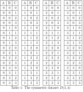
m different values. We denote the dataset asD(K, m). The master table contains all the possible entries by taking different values over K attributes. Hence, the number of rows in the master table ismK. Under this definition, the dataset with a symmetric structure, is thus called symmetric synthetic dataset.

For example, assume dataset D(3,4) has 3 attributes A,B and C. Each attribute takes four values 0, 1, 2 or 3. The master table has 64 (= 43) entries. And the master table is shown in Table 1.

2.2 Views of symmetric synthetic dataset

A view, as a common type of derived data, is a virtual table consists of the result

set of a query. In this context, we denote a view by its associated attributes. In a synthetic dataset D(K, m), there are 2K _{diﬀerent associated views. Evaluate the size}

(2)

V2, then they have identical size. And if view V1 is a decedent of view V2, then V2 is

at least m times the size ofV1.

For example, D(3,4) has 8 (=23_{) views.} _{Each view which contains only one}

attribute (view {A}, {B} or {C}) has 4 (= 41_{) rows, shown in Table 2. And each}

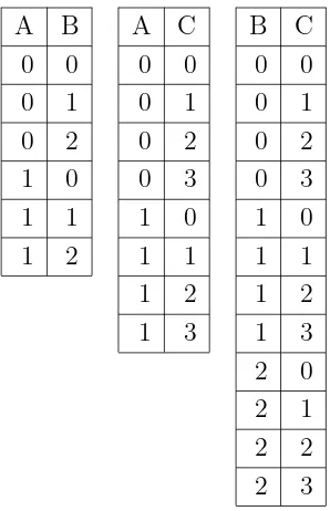
view which contains two attributes (view {A, B}, {B, C} or {A, C}) has 16 (= 42₎

rows, shown in Table 3. And the raw-data view (view{A, B, C}) has 64 (= 43_{) rows.}

View{A, B}is four times the size of view {A}.

The size of views inD(4,7) andD(5,9) are shown in Table 4 and Table 5, respec-tively.

3 Non-symmetric synthetic dataset

In this section, we deﬁne two types of non-symmetric synthetic dataset based on the the symmetric synthetic dataset obtained in the previous section.

3.1 Type I non-symmetric synthetic dataset

3.1.1 Construction

We consider a generalization of the symmetric synthetic datasets by changing the condition that all the attributes take identical number of values. Deﬁne a datasetDas follows. The datasetDhasKattributes, denoted asa1,a2, . . . , aK. Attributeaktakes

mk diﬀerent values, fork= 1,2, . . . , K. We denote the dataset asD(K;m1, . . . , mK).

The master table contains all the possible entries by taking diﬀerent values over K

attributes. We deﬁne dataset D(K;m1, . . . , mK) as type I non-symmetric synthetic

dataset. Hence, given the input parameters (K;m1, . . . , mK), we obtain the master

table of type I non-symmetric synthetic dataset with the number of rows ΠK k=1mk.

For example, assume dataset D(3; 2,3,4) has 3 attributesA, B and C. Attribute

Atakes two values 0 or 1; Attribute B takes three values 0, 1 or 2; Attribute C takes four values 0, 1, 2, or 3. The master table has 24 (= 2×3×4) entries. And the master table is shown in Table 6.

Note that we could obtain the input parameters (K;m1, . . . , mK) for a type I

non-symmetric dataset based on a symmetric synthetic datasetD(K, m) by randomly choosing a number mk from {1,2, . . . , m} as the number of values for each attribute

ak.

3.1.2 Views

The non-symmetric datasetD(K;m1, . . . , mK) has 2K diﬀerent associated views. We

(3)

its attribute. The size of view {ak1, ak2, . . . , akl}, measured by its number of rows, is mk1mk2· · ·mkl.

The views in a type I non-symmetric dataset lacks of symmetric properties while it has its own properties. Letmmin = min1≤k≤Kmk. Hence, ifV1 is a descendent ofV2

in the view lattice of D(K;m1, . . . , mK),V2 is at leastmmin times the size ofV1. And

identical number of attributes in diﬀerent views does not guarantee identical size of them.

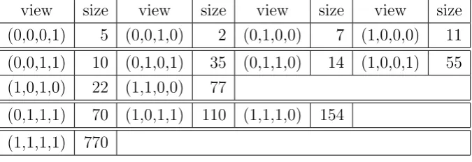
For example, D(3; 2,3,4) has 8 (= 23_{) views. As shown in Table 7, view}_{_A_}_,_{_B_}

and {C}has 2, 3 and 4 rows, respectively. And view {A, B},{A, C}and {B, C} has 6 (= 2×3), 8 (= 2×4) and 12 (= 3×4) rows, respectively, shown in Table 8. The raw-data view has 24 rows. View {A, B} is three times the size of view{A}.

The size of views in D(4; 5,2,7,11) and D(5; 6,8,5,13,7) are shown in Table 9 and Table 10, respectively.

3.2 Type II non-symmetric synthetic dataset

3.2.1 Construction

The type I non-symmetric dataset lacks of symmetric properties while it has its own special structure in the master table and views. We consider to break such properties in a new dataset, so-called type II non-symmetric synthetic dataset, by partially eliminating rows from the master table of a type I non-symmetric synthetic dataset obtained in the previous section.

The easy way to do the elimination is to randomly eliminating each row in a type I non-symmetric synthetic dataset with a certain probability. However, after conducting this elimination on some datasets, we observe that the size of views in the new datasets does not change much. Thus, we derive the following elimination procedure for obtaining a type II non-symmetric synthetic dataset.

Given a type I non-symmetric synthetic datasetD(K;m1, . . . , mK) with attributes

a1, . . . , aK, we conduct an elimination process based from attribute a1 toaK. To do

this, for each attributeak, the sub-elimination process consists of two steps. We ﬁrst

do elimination from the ﬁrst row of the master table to the end. Assume each row in the master table ofD(K;m1, . . . , mK) would be kept with an identical probability

pk, and equivalently, eliminated with probability qk = 1− pk. Secondly, for each

eliminated rowr, we also eliminate the rows in the master table with the same values as r on all attributes except ak.

Let us denote byS0 the number of rows in the master table ofD(K;m1, . . . , mK).

S0 = ∏K

k=1mk. In order to evaluate the expected number of rows remaining in

(4)

table into ∏K_k₌₂mk groups, such that the rows in each group have identical values

over a2, . . . , aK, and are diﬀerent from each other only on the value of attribute a1.

In other words, each group corresponds to one row in view {a2, a3, . . . , aK}. And the

number of rows in each group is m1, which refers to the number of values on a1. If

one row is eliminated at the ﬁrst step of the sub-elimination process, all the rows in its group are eliminated at the second step. In other words, each group of rows will be eliminated or remaining in the master table simultaneously. And the probability of eliminating the whole group of rows is 1−pm1

1 . Thus, the expected number of rows

in each group remaining in the master table is m1pm1 1. And the expected number

of rows remaining in the master table after the elimination based on attribute a1,

denoted by S1, is

S1 = ∑

group

m1pm11 =m2· · ·mKm1pm11 =S0pm1 1

To evaluate the expected remaining rows after elimination based on attribute

a2, we reorder the remaining entries after elimination based on a1 grouped by a1, a3,

a4, . . . , aK. TheS1rows are divided intom1m3· · ·mK groups. The number of rows in

groupg, denoted bymg, is no more than m2, i.e., mg ≤m2,∀g. Thus, the probability

of eliminating all the rows in group g is 1−pmg

2 . And the expected number of rows

remaining in the master table after the elimination based on attributea2, denoted by

S2, is

S2 =

m1m∑3···mK

g=1

mgp mg

2 ≥

m1m∑3···mK

g=1

mgpm2 2 =S1pm22

Thus,

S2 ≥S0pm11p

m2

2

.

Similarly, we obtain the expected number after the sub-elimination process based on attribute ak, denoted by Sk, and

Sk ≥S0pm11p

m2

2 · · ·p

mk

k

And thus, the expected number of remaining rows after the whole elimination process, denoted by ¯S, satisﬁes

¯

S≥S0

K

∏

k=1

pmk

k = K

∏

k=1

mkpm_kk (1)

As a result, given the lower bound of the expected rows, after elimination in the master table, denoted by SL, we could choose the elimination probability qk for each

sub-elimination process based on attribute ak. The algorithm of obtaining a type II

(5)

I non-symmetric synthetic dataset D(K;m1, . . . , mK) is shown as follows.

Step 0. Input SL and D(K;m1, . . . , mK). Choosep1, . . . , pK such that

SL ≥

∏K i=1mip

mi

i . Set k= 1.

Step 1. Mark each row in the current table as ’selected’ with probability 1−pk.

(If a row is marked, it will be eliminated.)

Step 2. Order the rows in the current table grouped by attribute a1, a2, . . ., ak−1,

ak+1,. . ., aK.

For g = 1 to ∏K_i₌₁mi

/

mk

In each group g, if there exists one row marked, then mark all themk rows

in that group.

Step 3. Eliminate all the marked rows in the table. Ifk =K, output the table as

D′, otherwise k=k+ 1 and go to step 1.

3.2.2 Views

After the new master table is obtained, all the views will be redeﬁned. Thus, we could not guarantee that the views with identical number of attributes have identical size. And the relationship between the size of view and the number of values in each of its attribute is no longer established.

4 Conclusions

In this report, we have deﬁned a symmetric synthetic dataset and two kinds of non-symmetric synthetic dataset. The views of the non-symmetric synthetic datasets have some symmetric properties while the non-symmetric dataset may not. Once the input parameters for dataset construction are given, the type I non-symmetric synthetic dataset is a deterministic set while the type II non-symmetric dataset is a random one. All these datasets are beneﬁcial for testing the algorithms in computational experiments such as models in Asgharzadeh[1].

References

(6)

Appendix

A B C A B C A B C A B C

0 0 0 1 0 0 2 0 0 3 0 0

0 0 1 1 0 1 2 0 1 3 0 1

0 0 2 1 0 2 2 0 2 3 0 2

0 0 3 1 0 3 2 0 3 3 0 3

0 1 0 1 1 0 2 1 0 3 1 0

0 1 1 1 1 1 2 1 1 3 1 1

0 1 2 1 1 2 2 1 2 3 1 2

0 1 3 1 1 3 2 1 3 3 1 3

0 2 0 1 2 0 2 2 0 3 2 0

0 2 1 1 2 1 2 2 1 3 2 1

0 2 2 1 2 2 2 2 2 3 2 2

0 2 3 1 2 3 2 2 3 3 2 3

0 3 0 1 3 0 2 3 0 3 3 0

0 3 1 1 3 1 2 3 1 3 3 1

0 3 2 1 3 2 2 3 2 3 3 2

0 3 3 1 3 3 2 3 3 3 3 3

Table 1: The symmetric datasetD(3,4)

A B C

0 0 0

1 1 1

2 2 2

3 3 3

(7)

A B A C B C

0 0 0 0 0 0

0 1 0 1 0 1

0 2 0 2 0 2

0 3 0 3 0 3

1 0 1 0 1 0

1 1 1 1 1 1

1 2 1 2 1 2

1 3 1 3 1 3

2 0 2 0 2 0

2 1 2 1 2 1

2 2 2 2 2 2

2 3 2 3 2 3

3 0 3 0 3 0

3 1 3 1 3 1

3 2 3 2 3 2

3 3 3 3 3 3

Table 3: View {A, B}, {A, C}and {B, C}in the symmetric dataset D(3,4)

view size view size view size view size (0,0,0,1) 7 (0,0,1,0) 7 (0,1,0,0) 7 (1,0,0,0) 7

(0,0,1,1) 49 (0,1,0,1) 49 (0,1,1,0) 49 (1,0,0,1) 49

(1,0,1,0) 49 (1,1,0,0) 49

(0,1,1,1) 343 (1,0,1,1) 343 (1,1,1,0) 343

(1,1,1,1) 2401

Table 4: Sizes of views inD(4,7)

view size view size view size view size view size

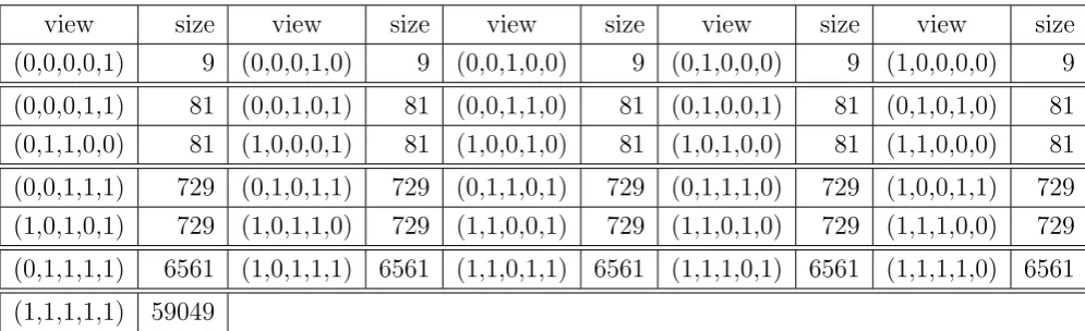
(0,0,0,0,1) 9 (0,0,0,1,0) 9 (0,0,1,0,0) 9 (0,1,0,0,0) 9 (1,0,0,0,0) 9

(0,0,0,1,1) 81 (0,0,1,0,1) 81 (0,0,1,1,0) 81 (0,1,0,0,1) 81 (0,1,0,1,0) 81

(0,1,1,0,0) 81 (1,0,0,0,1) 81 (1,0,0,1,0) 81 (1,0,1,0,0) 81 (1,1,0,0,0) 81

(0,0,1,1,1) 729 (0,1,0,1,1) 729 (0,1,1,0,1) 729 (0,1,1,1,0) 729 (1,0,0,1,1) 729 (1,0,1,0,1) 729 (1,0,1,1,0) 729 (1,1,0,0,1) 729 (1,1,0,1,0) 729 (1,1,1,0,0) 729

(0,1,1,1,1) 6561 (1,0,1,1,1) 6561 (1,1,0,1,1) 6561 (1,1,1,0,1) 6561 (1,1,1,1,0) 6561

(1,1,1,1,1) 59049

(8)

A B C A B C 0 0 0 1 0 0 0 0 1 1 0 1 0 0 2 1 0 2 0 0 3 1 0 3 0 1 0 1 1 0 0 1 1 1 1 1 0 1 2 1 1 2 0 1 3 1 1 3 0 2 0 1 2 0 0 2 1 1 2 1 0 2 2 1 2 2 0 2 3 1 2 3

Table 6: Non-symmetric dataset D(3; 2,3,4)

A B C

0 0 0

1 1 1

2 2

3

Table 7: View {A},{B}and {C} in the non-symmetric dataset D(3; 2,3,4)

A B A C B C

0 0 0 0 0 0

0 1 0 1 0 1

0 2 0 2 0 2

1 0 0 3 0 3

1 1 1 0 1 0

1 2 1 1 1 1

1 2 1 2 1 3 1 3 2 0 2 1 2 2 2 3

(9)

view size view size view size view size (0,0,0,1) 5 (0,0,1,0) 2 (0,1,0,0) 7 (1,0,0,0) 11

(0,0,1,1) 10 (0,1,0,1) 35 (0,1,1,0) 14 (1,0,0,1) 55 (1,0,1,0) 22 (1,1,0,0) 77

(0,1,1,1) 70 (1,0,1,1) 110 (1,1,1,0) 154

(1,1,1,1) 770

Table 9: Sizes of views in D(4; 5,2,7,11)

view size view size view size view size view size (0,0,0,0,1) 6 (0,0,0,1,0) 8 (0,0,1,0,0) 5 (0,1,0,0,0) 13 (1,0,0,0,0) 7

(0,0,0,1,1) 48 (0,0,1,0,1) 30 (0,0,1,1,0) 40 (0,1,0,0,1) 78 (0,1,0,1,0) 104

(0,1,1,0,0) 65 (1,0,0,0,1) 42 (1,0,0,1,0) 56 (1,0,1,0,0) 35 (1,1,0,0,0) 91

(0,0,1,1,1) 240 (0,1,0,1,1) 624 (0,1,1,0,1) 390 (0,1,1,1,0) 520 (1,0,0,1,1) 336

(1,0,1,0,1) 210 (1,0,1,1,0) 280 (1,1,0,0,1) 546 (1,1,0,1,0) 728 (1,1,1,0,0) 455

(0,1,1,1,1) 3120 (1,0,1,1,1) 1680 (1,1,0,1,1) 4368 (1,1,1,0,1) 2730 (1,1,1,1,0) 3640

(1,1,1,1,1) 21840