MAXIMIZING
NETWORK
LIFETIME
USING
ROUTING
ALGORITHM FOR WIRELESS SENSOR NETWORK
Sathyanarayana1
1. INTRODUCTION
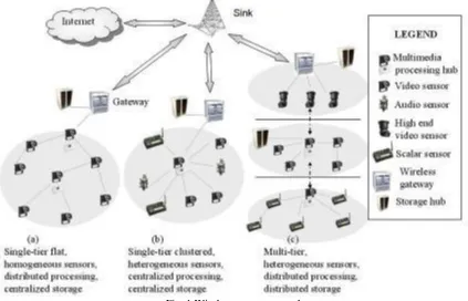
A Wireless Sensor Network or WSN is supposed to be made up of a large number of sensors and at least one base station. The sensors are autonomous small devices with several constraints like the battery power, computation capacity, communication range and memory. They are also supplied with transceivers to gather information from its environment and pass it on up to a certain base station, where the measured parameters can be stored and available for the end user. Fig 1 shows the structure of wireless sensor network.
Fig. 1 Wireless sensor networks
1
Assistant Professor, Department of Computer Science & Engineering, J N N College of Engineering, Shivamogga, Karnataka, India
International Journal of Latest Trends in Engineering and Technology
Vol.(14)Issue(1), pp.041-047
DOI: http://dx.doi.org/10.21172/1.141.08
e-ISSN:2278-621X
2. PROBLEM STATEMENT
The main limitation of WSNs is that the sensor nodes are operated on limited power sources. If the distance between source and the destination is too long, it will consume more energy. Thus, one of the most challenging issues in WSNs is energy conservation of the sensor nodes to maximize the network lifetime.
3. REQUIREMENT ANALYSIS AND DESIGN
Requirement analysis is critical to the success or failure of a system or software project. The requirements should be documented, actionable, measurable, testable, traceable, related to identified business needs or opportunities, and defined to a level of details sufficient for system design.
3.1 Sensor Node Configuration
Sensor node deployment is one of the critical topics addressed in wireless sensor networks (WSNs) research, which determines coverage efficiency of WSNs. Mobile sensor network is made up of group/groups of small low-power sensor nodes that can sense specific situations or collect information, and then transmit that information to sink nodes using wireless ad hoc communication. Several nodes with various kinds of sensors for sound, heat, magnetic field, and infrared ray are randomly scattered in a target area. These sensors move, voluntarily avoiding obstacles and other nodes, establish sensing coverage and configure their communication network.
Target area is the field where sensor nodes are deployed. Here 600x600 meter square target area is considered. In this range the sensor nodes are deployed.
3.2 Functional Requirements
The functional requirements considered in this project are as follows:
Communication range: The range in which the sensor nodes communicate. Here we consider 250m of communication range.
Sensing range: It is the range within which the required activities are sensed by the sensor nodes. Here we consider 3.65262e-10m of sensing range.
Data routing: UDP is established and datagrams are transmitted. UDP (User Datagram Protocol) is an alternative communications protocol to Transmission Control Protocol (TCP) used primarily for establishing low-latency and loss tolerating connections between applications on the Internet. ... Both protocols send short packets of data, called datagrams.
Cluster head: Each cluster has a coordinator called cluster head. It involves grouping of sensor nodes into clusters and electing cluster heads (CHs) for all the clusters. CHs collect the data from respective cluster's nodes and forward the aggregated data to base station. A major challenge in WSNs is to select appropriate cluster heads.
Cluster members: Nodes other than cluster head in a cluster is called cluster members. A Node can belong to at most one Cluster at any time. A node is referred to as an orphan node when it doesn't belong to any cluster. A node can be made a member of cluster when creation or you can change the cluster membership after the cluster and the node have been created.
3.3 Non-Functional Requirements
The non-functional requirements considered in this project are as follows:
Network Lifetime (NLT): The network lifetime (NL) of the WSN is defined as the number of rounds until the first node dies (FND). For the sake of completeness, we also show the number of alive sensor nodes per round.
Power imbalance factor (PIF): This metric is defined to evaluate the energy balance characteristics of the proposed algorithm.
Energy Consumption: The energy consumption is the sum of used energy of all the nodes in the network, where the used energy of a node is the sum of the energy used for communication, including transmitting, receiving, and idling.
Throughput: Throughput is the maximum rate of production or the maximum rate at which something can be processed. A benchmark can be used to measure throughput. In data transmission, network throughput is the amount of data moved successfully from one place to another in a given time period, and typically measured in bits per second (bps), as in megabits per second (Mbps) or gigabits per second (Gbps).
3.4 System Architecture
Fig 2. System Architecture
The fig 2 shows the overall system architecture. The architecture is divided into two phases, namely, node deployment and clustering-routing. In the node deployment phase, the nodes are deployed randomly in the defined target area. Next, the clustering takes place based on the distance of nodes from the base station. Then, the cluster head selection takes place in every cluster based on the residual energy. After the clustering and cluster head selection process, the source node is assigned randomly. Then routing is established using AODV protocol to send datagrams from source to base station.
4. IMPLEMENTATION
This section explains the design and implementation of maximizing the lifetime of wireless sensor networks using energy aware routing protocol using algorithms and flowcharts.
Node Deployment: The type of nodes used here are mobile nodes. These nodes are deployed randomly in a defined area. All nodes are initially given a certain amount of energy. The deployment of nodes is implemented according to the flowchart given in the fig 3.
Algorithm: Step 1: Deploy.
Step 2: Set the position for base station. Step 3: Set the location for remaining nodes. Step 4: End deploy
Fig. 3 Flowchart for Node Deployment
Clustering: Clustering is done based on the location of base station. Each cluster has a cluster head (CH) and cluster members (CM). Each sensor node sets its own timer independently before it starts the campaign for CH selection. Let t(i) be the timer of sensor node i which is derived as follows
(4.1)
Algorithm:
Step 1: Start clustering.
Step 2: Calculate distance from every node to every other using distance formula. Step 3: Divide area into 4 regions based on the location of base station.
Step 4: Assign different colors for nodes in different regions. Step 5: Calculate residual energy of each node.
Step 6: Sort the nodes in the increasing order of their residual energy using bubble sort. Step 7: Select the node with highest residual energy as cluster head.
Step 8: Assign color for cluster head. Step 9: Select source node.
Step 10: Assign color for source node.
Step 11: Set up UDP Agent, Null Agent, CBR traffic. Step 12: End clustering.
Simulation: Ns is a discrete event simulator targeted at networking research. Ns provide substantial support for simulation of TCP, routing and multicast protocols over wired and wireless networks.
Here we are using NS-2 simulator. Ns2 stands for network simulator version 2. It is an open source event-driven simulator designed especially for research in computer communication networks.
The parameters used in simulation are shown in the table 4.1. Parameter name Parameter value
Number of nodes 25,50,100,150,200
Communication Range 250 m
Initial Energy 1J
Receiving Power (rx) 1.0mW
Transmission Power (tx) 3.0mW
Table 4.1 Parameters used
5. RESULTS AND ANALYSIS
The proposed energy aware routing protocol is written in Tcl and simulated using Ns-2. In this section, we present the results of the simulation and also the comparisons with the existing protocols, DSDV and DSR. The snapshots of the previously discussed modules are presented in this section.
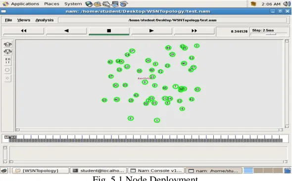
Node Deployment: Here, the nodes are deployed in given target area. The fig 5.1 shows the node deployment
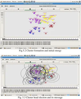
Cluster Formation and assigning initial energy: Here, cluster is formed based on the location of nodes and initial energy is assigned to all the nodes. The fig 5.2 shows the cluster formation and initial energy.
Cluster head selection and broadcasting CH elected message to its CMs: Here, Cluster head is elected according to the residual energy of the nodes and send its elected message to its cluster members. The fig 5.3 shows the cluster head election and its message
Fig.5.2 Cluster formation and initial energy
Fig. 5.3 Cluster head election and its message
Sending datagrams to the base station: Here, datagrams are sending from the source node to the base station through cluster heads. The fig 5.4 shows sending datagrams to the base station.
Performance evaluation: In order to evaluate the performance of the AODV routing protocol for various density of the sensor nodes, number of nodes are varied from 10 to 100 in the same target area.
Here, we have considered four performance metrics. Namely, delay, throughput, packet delivery ratio (pdr) and average energy consumption. The fig 5.5 and fig 5.6 shows the variation of delay and throughput as the number of nodes are varied respectively. We can observe that as the number of nodes increases, delay and throughput also increases.
Fig. 5.5 Number of nodes vs Delay Fig. 5.6 Number of nodes vs Throughput
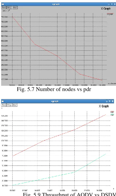
The figure 5.7 shows the variation of pdr when number of nodes are varied. We can observe that as the number of nodes increase, the packet delivery ratio decreases due to excessive packet drop that might occur due to congestion. The figure 5.8 shows the variation of average energy consumption when the number of nodes are varied. We can see that as the number of nodes increase, the average energy consumption decreases. The graph in the fig 5.9 shows the comparison between the throughput of AODV and DSDV. In DSDV, throughput decreases because of periodic routes information updates and if the node mobility is at high speed. In AODV, throughput is stable because it don’t broadcast any routing information. The fig 5.10 shows the comparison between the average energy consumption in AODV and DSDV. In this, we can observe that DSDV consumes more energy than AODV.
Fig. 5.7 Number of nodes vs pdr Fig. 5.8 Number of nodes vs Energy
6. CONCLUSION
The energy efficient routing protocol, AODV has been used to minimize the energy consumption and increase the network lifetime in wireless sensor network. Here the algorithm is implemented for clustering and cluster head selection process. Using the AODV routing protocol, the simulation in ns-2 using tcl script is done. By considering the performance metrics such as throughput, delay, packet delivery ratio (pdr) and average energy consumption the graph is plotted by varying the number of nodes. The efficiency of AODV protocol is analyzed by comparing the throughput and average energy consumption of AODV and DSDV protocol. The analysis of result shows that the AODV protocol is more efficient than DSDV as it consumes less energy and hence network lifetime is maximized when AODV protocol is used.
7. REFERENCES
[1] Muhammad R Ahmed, Xu Hung, Dharmandra Sharma, and Hongyan Cui, “Wireless Sensor Network: Characteristics and Architectures”, Vol: 6, No: 12, 2012.
[2] Manal Abdullah, Aisha Ehsan, “Routing Protocols for Wireless Sensor Networks: Classifications and Challenges”, Vol: 2, 2014.
[3] Gulfishan Firdose Ahmed, Raju Barskar, and Nepal Barskar, “An Improved DSDV Routing Protocol For Wireless Sensor Networks”, ICCCS-2012. [4] Taewook Kang, Jangkyu Yun, Kijun Han, “A Clustering Method for Energy Efficient Routing in Wireless Sensor Networks”, 2007.
[5] Varinder Pal Singh Sandhu, Saurabh Kumar, “Energy Efficient HEED protocol in wireless sensor networks”, 2015. [6] Tarachand Amgoth, Prasanta K. Jana., “Energy-aware routing algorithm for wireless sensor networks”, Vol: 41, 2015.